The following is the first section of the 1st Chapter of the "Advanced Dynamic Simulation Course". This course has been taught to engineers at Rockwell Automation, Ford Motor Co., and others. Reading through this first section is a great way to brush up on Laplace transforms, using them to solve differential equations, and applying these methods to control system design, using Bode Plot methods.
This chapter covers fundamentals of Industrial Control System Analysis, Control System Stability, and Laplace Transforms. For Control System Engineers
CHAPTER 1
FUNDAMENTALS
1.1. Review of complex numbers and complex algebra
1.1.1 Introduction
Why start this course work with a review of complex numbers? Because classical control system analysis is based on the application of complex variables and functions of complex variables. And complex variables in turn are functions of complex numbers.
The analysis of ac circuits can also use complex numbers. For example, sinusoidal signals are often transformed into phasors, and resistance, capacitance, and inductance are often transformed into impedance. These complex variables -- phasors and impedance -- are complex numbers.
Complex numbers must be manipulated using complex algebra, which is an extension of the algebra of real numbers. This is because complex numbers have their own special rules for adding, subtracting, multiplying, and dividing.
Some of the complex arithmetic is avoided, however, when using the Laplace transformation technique as part of the control system analysis. When using the technique, the differential equations (describing the system to be controlled) are converted into algebraic equations which are functions of a complex variable ( s = s
+ jw
). Then ordinary algebra can be used to manipulate the equations into forms more suited for factoring and/or plotting the roots in the complex plane.
1.1.2 Imaginary Numbers
Imaginary numbers were invented to provide solutions to square roots of negative numbers. They have an unfortunate name, because they exist more than in the imagination. There is no one universally accepted way of writing them. In the electrical field, however, it is standard practice to use the letter j , as in j2 , j0.01 , and -j5.6.
Imaginary numbers sometimes require special rules when combining them:
- Adding and subtracting
use the same rules as those for real numbers.
- Examples: j2 + j0.01 = j2.01
j2 - j5.6 = -j3.6.
- Multiplying
two imaginary numbers, however, uses a different rule than that for real numbers. It results with a real number whose sign is opposite of what you would get if they were real numbers.
- Examples: (j2)(j0.01) = -0.02
(j2)(-j5.6) = +11.2.
- Dividing
two imaginary numbers also uses a different rule. It results with in a real number, but in this case the sign is the same as you would get if they were real numbers.
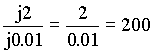
- Examples: (j2) / (j0.01) = 200
(-j5.6) / (j2) = -2.8.
These rules for multiplying and dividing imaginary numbers may be easier to remember if you view the j operator at being equal to Ö
-1. Then, j2 = -1. For instance, the examples given above can be viewed in the following ways:


This view of j should be used as a memory aid only, because j is not a number itself; it just designates a number as being imaginary.
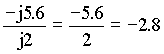
Division involving a real and an imaginary number involves a special step, called rationalizing, whenever the imaginary number is in the denominator. For example,
The rationalizing step was when the numerator and denominator were each multiplied by j.
1.1.3 Complex numbers
1.1.3.1 Rectangular Form of a Complex Number
When a real number and an imaginary number are added or subtracted, as in 12 + j5 and -4 + j3 , the result is a complex number in rectangular form. A complex number is a point on the complex plane shown in Figure 1.1.1.
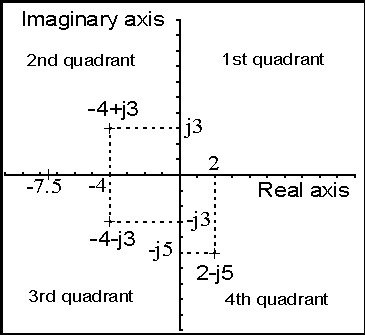
Figure 1.1.1 Complex plane represents complex numbers as points
The following conventions pertain to the complex plane in Figure 1.1.1:
- The horizontal axis in the complex plane is called the real axis.
- The vertical axis is called the imaginary axis.
- The horizontal and vertical axes divide the complex plane into four
quadrants. Regarding the points (complex numbers) shown in Figure 1.1.1:
- (-4 + j3) lies in the 2nd quadrant,
- (-4 - j3) lies in the 3rd quadrant,
- (2 - j5) lies in the 4th quadrant,
- one lies on the negative real axis (at -7.5) .
Some other complex-plane notation we will deal with when performing control system analyses are:
The left-half plane ; i.e., to the left of the imaginary axis. In addition, points not on the real axis will always appear in complex conjugate pairs. Such pairs, as
(-4+j3) and (-4-j3)
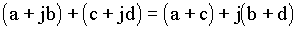
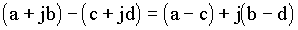
in the figure, have the same negative real part and, except for the sign, the same imaginary part. The rectangular form is practical only for adding and subtracting, as indicated in the following:
- Adding and subtracting
operations are applied separately to the real and imaginary parts. For example,
- Multiplying
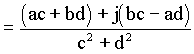
two complex numbers in rectangular form follow the ordinary rules of algebra, along with the rules for imaginary numbers. For example,
 = (ac-bd) +j(ad+bc) = (ac-bd) +j(ad+bc)
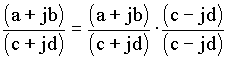
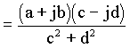
- Dividing
two complex number in rectangular form is a two-step process:
- rationalize the denominator (i.e., make it real) by multiplying the top and bottom by the complex conjugate of the denominator;
- then simplify. For example,
1.1.3.2. Exponential and Polar Forms of a Complex Number
The exponential and polar forms are summarized below. The polar form is a shorthand way of writing the exponential form. Its simplicity makes it much more popular
- The exponential form of a complex number is Aejq
where: A is the magnitude
q
is angle
The basis of these forms is Euler’s identity for complex numbers:
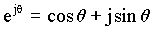
Figure 1.1.2 shows how a complex number -- e.g., (-4 + j3) -- can be expressed in exponential and polar forms.
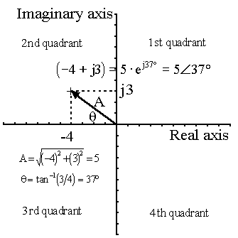
Figure 1.1.2 Exponential and polar forms require magnitude (A) and angle (q
)
The magnitude A is found from the right-triangle rule:
(hypotenuse, c)2 = (side, a)2 + (side, b)2
The angle is found from studying Euler’s identity and noting that:
tanq
= (imaginary part) / (real part)
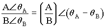
The exponential and polar forms are most practical for multiplying and dividing.
- Multiplying two complex numbers
- in exponential form (use the law of exponents):
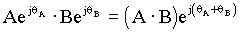
- in polar form: multiply the amplitudes and add the angles; i.e.,
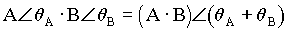
- Dividing
two complex numbers
- in exponential form (use the law of exponents):
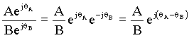
- in polar form: divide the amplitudes and subtract the angles:
1.2. Definition of a Linear System
1.2.1. Math Models of Physical System
Deriving a reasonable (mathematical) model of the physical system is perhaps the most important part of an analysis effort. There are many different forms in which the model can be developed. The model choice should be the one most suitable for the particular system and circumstances.
State-space models, for example, are most suitable for optimal control problems, multiple-input, multiple-output (MIMO) systems, and for computer-aided design algorithms (e.g., MATLAB). Transfer-function models, on the other hand, are most suitable for analyzing the transient or frequency response of single-input, single-output (SISO) time-invariant systems.
1.2.2. Simplicity vs Accuracy
Generally, the accuracy of an analysis is improved only at the cost of increased model complexity. The linear lumped-parameter model of a physical system, for example, ignores nonlinear effects and distributed parameters. As a result, it may be valid only at low frequencies, since the ignored distributed parameters typical produce high-frequency effects.
The recommended approach is to start with a simple model. Perform some analyses or generate some solutions to get a feeling for the accuracy of the modelling. Perhaps the simple model was sufficient for the analysis objectives at hand. If not, then build a more complex model to improve on the solution.
1.2.3. Linear Systems
A linear model of a physical system, from a mathematical view point, generally means the principle of superposition applies; i.e., the response of the model to several inputs equals the sum of the responses to each input taken alone. Using this principle, a complicated solution to a linear differential equation can be built up from a series of simple solutions.
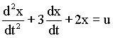
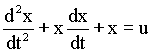
A differential equation -- the basis of control system modelling -- is linear if the coefficients are constants or functions of the independent variable. An example differential equation with constant (i.e., time-invariant) coefficients is
 (1.2.1) (1.2.1)
An example differential equation with a coefficient that is a function of the independent variable (i.e., time) is
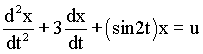 (1.2.2) (1.2.2)
1.2.4. Nonlinear Systems
A nonlinear model of a physical system is one in which the principle of superpostion does not apply. The response to two inputs, for example, will not equal the sum of the response with each input taken alone.
Some examples of nonlinear effects in physical systems, which can be successfully modelled to various degrees, are listed below:
- Saturation (with large signals)
- Dead space or backlash (affecting small signals)
- Power-law dependence (e.g., damping force vs velocity)
- Frequency-dependent dampers (linear at low frequencies, nonlinear at high frequencies)
Figure 1.2.1 shows the characteristic curves for the first three nonlinearities above.
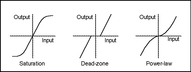
Figure 1.2.1 Characteristics curves for various nonlinearities
One way a differential equation becomes nonlinear is if the coefficients are functions of the dependent variable. For example,
 (1.2.3) (1.2.3)
The other way a differential equation becomes nonlinear is if the order of the dependent variable and/or its derivative(s) is greater than one. For example,
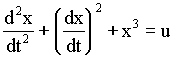 (1.2.4) (1.2.4)
Since all physical systems are to some degree nonlinear, a truly linear model does not really exist. There typically will be a limited range of output magnitudes, however, over which the response of the linear model approximates sufficiently well the real world.
If no limited linear range exists, usually the nonlinear equations can be linearized around an operating (equilibrium) point. The result is a linear system approximately equivalent to the nonlinear system within a limited operation range. The linearization technique is very important in control engineering.
1.3. The Laplace Transform
This section reviews the Laplace transform method for solving linear differential equations. The following features makes the method attractive for control system analysis:
- The method converts differentiation (and integration) and many common functions -- such as steps, ramps, sinusoids, and exponentials -- into algebraic terms in a complex variable s .
- The transformed differential equation is an algebraic equation which can be solved for the dependent variable.
- The solution (as a function of time) of the differential equation -- i.e., the inverse Laplace transform -- may be then found directly from a Laplace transform table, or by first using the partial fraction technique and then the transform table.
Often the final step of finding the inverse Laplace transform is not necessary. Graphical techniques -- e.g., Bode plot, root locus diagram, Nyquist plot, and Nichols chart -- exists for predicting the system performance without actually finding the differential equation solution as a function of time.
1.3.1 Notation
The notation conventionally used in the Laplace transform includes the following:
- f(t) = a function of time t such that f(t) = 0 for t < 0
- s = complex variable
 (1.3.1) (1.3.1)
- s
= real part
- w
= imaginary part
- L = an operational symbol indicating the Laplace transform
- F(s) = Laplace transform of f(t)
- definition of the Laplace transform of f(t)
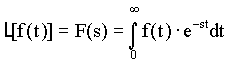 (1.3.2) (1.3.2)
- notation for the inverse Laplace transform
 (1.3.3) (1.3.3)
1.3.2 Some Useful Properties
Some useful properties and results of the Laplace transform are as follows:
- multiplying by a constant A
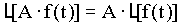 (1.3.4) (1.3.4)
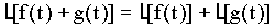 (1.3.5) (1.3.5)
- transform of the 1st derivative
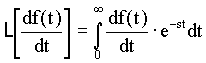 (1.3.6) (1.3.6)
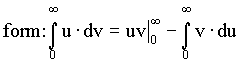 (1.3.7) (1.3.7)
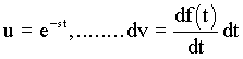 (1.3.8) (1.3.8)
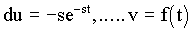 (1.3.9) (1.3.9)
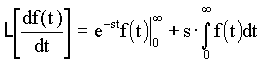 (1.3.10) (1.3.10)
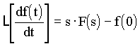 (1.311) (1.311)
- transform of the 2nd derivative (integrate by parts twice)
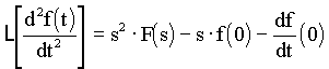 (1.3.12) (1.3.12)
- transform of the exponential function
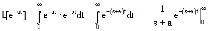 (1.3.13) (1.3.13)
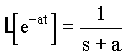 (1.3.14) (1.3.14)
- transform of a step function (amplitude = A)
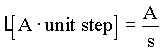 (1.3.15) (1.3.15)
1.3.3 Some Common Transform Pairs
Table 1.3.1 shows Laplace transforms of time functions that frequently appear in linear control system analysis.
| |
f(t) |
F(s) |
|
1 |
Unit impulse, d
(t) |
1 |
|
2 |
Unit step, U(t) |

|
|
3 |
t |

|
|
4 |

|

|
|
5 |

|

|
|
6 |
sin w
t |

|
|
7 |
cos w
t |

|
|
8 |
|
|
|
9 |
|
|
|
10 |
|
|
|
11 |
|
|
|
12 |
K* = complex conjugate of K |
|
Table 1.3.1 Laplace Transform Pairs
1.3.4 Example Application: First-Order Differential Equation Solution
As an application in which the Laplace transform is used to solve linear differential equation, consider the simple electrical network in Figure 1.3.1. Assume we want to solve for the current i(t) in the series RL circuit, immediately after it is connected together. The initial current, therefore, is zero; i.e., I(0) = 0 .
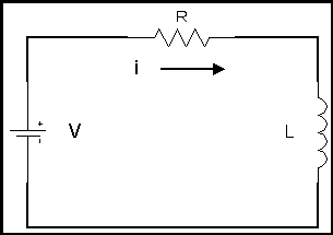
Figure 1.1.3 Series RL electrical circuit
The sum of the voltage drops around the series circuit equals the applied source voltage; i.e.,
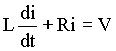 (1.3.16) (1.3.16)
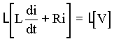
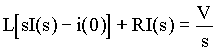
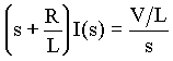
Taking the Laplace transform of both sides of the above equation and solving for the current yields:
 (1.3.17) (1.3.17)
 (1.3.18) (1.3.18)
 (1.3.19) (1.3.19)
 (1.3.20) (1.3.20)
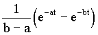
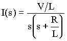
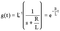
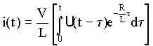
The time solution i(t) is the inverse Laplace transform I(s) ;..i.e.,
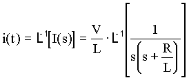 (1.3.21) (1.3.21)
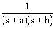
The Laplace transform on the right-hand side of Eq.(1.3.17) can be found in Table 1.3.1, namely the transform pair numbered 5. The time solution can therefore be written directly from the table:
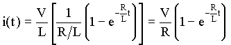 (1.3.22) (1.3.22)
Whenever the inverse Laplace transform is not readily known or available in the table of transform pairs on hand, it is sometimes necessary to first expand function into partial fractions -- simple rational functions of s for which the inverse Laplace is readily available. Using the I(s) expression above in Eq.(1.3.20) as an example, the right-hand side is expanded as follows:
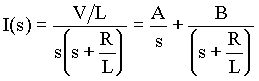 (1.3.23) (1.3.23)
Thus, we have two partial fractions, with coefficients A and B, which correspond to transform pairs numbered 2 and 4 in Table 1.3.1 . Rewriting the right-hand side of the above equation over a common denominator results in the following:
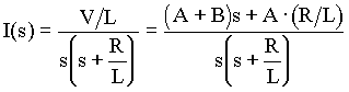 (1.3.24) (1.3.24)
The two numerators above must be equal. Comparing coefficients of s :
 (1.3.25) (1.3.25)
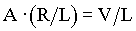 (1.3.26) (1.3.26)
Therefore,
 (1.3.27) (1.3.27)
 (1.3.28) (1.3.28)
Rewriting Eq.(1.3.20) in terms of the partial fractions:
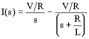 (1.3.29) (1.3.29)
Using Table 1.3.1
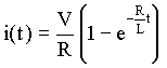 (1.3.30) (1.3.30)
as in Eq.(1.3.22).
1.3.5 More Useful Properties
 (1.3.31) (1.3.31)
 (1.3.32) (1.3.32)
 (1.3.33) (1.3.33)
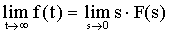
1.3.5.1 The final-value theorem
Equation (1.3.31) is a way to predict the steady-state (i.e., final value) of the solution from the Laplace transform, without the need to find the inverse transform. For example, in the RL circuit considered above, Eq.(1.3.22) and Eq.(1.3.30) indicate that in the steady-state -- i.e., in the limit as t ®
¥
-- the current Iss = V / R . This result may be obtained from the I(s) expression in Eq.(1.3.20) by applying the final-value theorem:
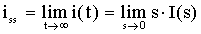 (1.3.34) (1.3.34)
 (1.3.35) (1.3.35)
 (1.3.36) (1.3.36)
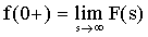
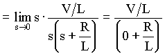
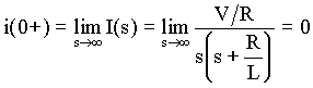
1.3.5.2 The initial-value theorem
Equation (1.3.32) allows us to predict the initial value of the variable an infinitesimally small time after the start of the solution (at t = 0+ ). For the RL circuit problem, we again start with the I(s) expression in Eq.(1.3.20) and apply the initial-value theorem:
 (1.3.37) (1.3.37)
as predicted by Eq.(1.3.22).
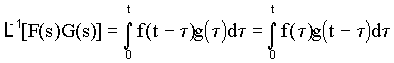
1.3.5.3 The convolution theorem
Equation (1.3.33) allows us to obtain the inverse Laplace transform by performing a special integration. Applying this to the RL circuit solution above, we start with the I(s) expression in Eq.(1.3.20) and, as with partial fractions, we look for a way to break I(s) into two simple factors -- F(s) and G(s) -- for which we know the inverse transform. For example,
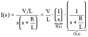 (1.3.38) (1.3.38)
Using Table 1.3.1:
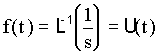 (1.3.39) (1.3.39)
 (1.3.40) (1.3.40)
From the convolution theorem:
 (1.3.41) (1.3.41)
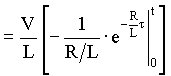 (1.3.42) (1.3.42)
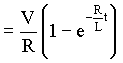 (1.3.43) (1.3.43)
as in Eq.(1.3.22).
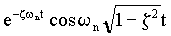
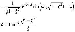
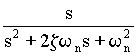
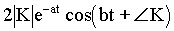
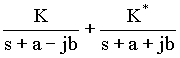
1.3.6 Inverse transform of complex conjugate pairs
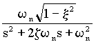
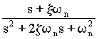
Another method for finding the inverse Laplace transform of F(s) that includes complex conjugate pairs is given in this portion of the supplement. The new transform pair developed below becomes entry #12 in Table 1.3.1 (at end of this discussion).
1.3.6.1 Form of F(s) with complex conjugate pairs
If the denominator of a Laplace transform has complex roots the following method may be employed to find the inverse Laplace transform.
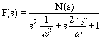 (1.3.44) (1.3.44)
This can be expressed in terms of its complex conjugate roots as:
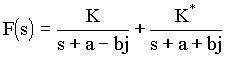 (1.3.45) (1.3.45)
Note: K is presented with respect to the positive conjugate pole. (i.e.  ) )
where:
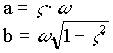 (1.3.46) (1.3.46)
1.3.6.2 Finding the values of K and K*
The value of K is found using the following substitution (follow the signs carefully)
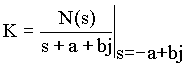 (1.3.47) (1.3.47)
similarly for 
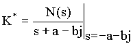 (1.3.48) (1.3.48)
will always be the conjugate of K, so no separate calculation is needed.
1.3.6.3 Form of the inverse transform
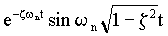
Once K and are known, the following rules are used to obtain the time solution:
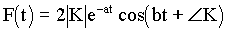 (1.3.49) (1.3.49)
The magnitude and angle of K are found using the rectangular to polar transformation presented in the section on complex numbers.
1.3.6.4 Using MATLAB to perform partial fraction expansion
When working with complex numbers it is very easy to make mistakes. The MATLAB program provides the user with a convenient method for performing partial fraction expansion. It is called the "residue" function. Briefly, here’s how to use it.
- define the numerator and denominator of the Laplace transform in terms of its polynomial coefficients. For example
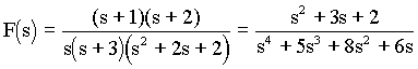 (1.3.50) (1.3.50)
- enter the numerator as a vector of numerator polynomial coefficients.
num=[1 3 2];
- enter the denominator as a vector of denominator polynomial coefficients
den= [1 5 8 6 0];
- use the residue function to find the partial fraction expansion coefficients.
The following is an excerpt from the MATLAB help screen for <residue>
[r,p,k]=residue(num,den); finds the residues, poles and direct term of a partial fraction expansion of the ratio of two polynomials, num(s) and den(s).
If there are no multiple roots,
num (s) r(1) r(2) r(n)
--------- = -------- + -------- + ... + -------- + k(s)
den (s) s - p(1) s - p(2) s - p(n)
Vectors [num] and [den] specify the coefficients of the polynomials in descending powers of s.
The following vectors are returned:
- residues in the column vector "r",
- pole locations in column vector "p",
- direct terms in row vector "k".
The number of poles: n = length(den)-1 = length(r) = length(p)
The direct term coefficient vector is empty if length(num) < length(den); otherwise length(k) = length(num)-length(den)+1
If p(j) = ... = p(j+m-1) is a pole of multiplicity m, then the expansion includes terms of the form
r(j) r(j+1) r(j+m-1)
-------- + ------------ + ... + ------------
s - p(j) (s - p(j))^2 (s - p(j))^m
[num,den] = residue(r,p,k), with 3 input arguments and 2 output arguments,
converts the partial fraction expansion back to the polynomials with coefficients [num] and [den].
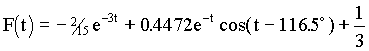
For the example given: (pasted directly from the MATLAB command window)
» num=[1 3 2];
» den= [1 5 8 6 0];
» [r,p,k]=residue(num,den);
r =
-2/15
-1/10 - 1/5i
-1/10 + 1/5i
1/3
p =
-3 0i
-1 + 1i
-1 - 1i
0 0i
k =
[]
From the "p" or pole vector we see that the second pole is the positive conjugate pole. Therefore the partial fraction expansion is given as:
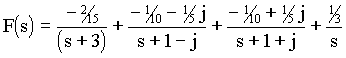 (1.3.51) (1.3.51)
We can find the rectangular to polar transformation of the residues in "r" with the following MATLAB commands
For Magnitude:
» abs(r)
ans =
0.1333
0.2236
0.2236
0.3333
For Phase:
» angle(r)*180/pi
ans =
180.0000
-116.5651
116.5651
0.0000
Using the rules presented above we can conclude that:
| 