APPLIED INDUSTRIAL CONTROL SOLUTIONS
ApICS LLC.
Accumulator Tower Tension Regulation
and
System Identification Techniques
B. T. BOULTER, H. W. FOX
© ApICS ® LLC 2000
ABSTRACT
Reports of tension and current major loop instabilities observed during the commissioning of a Hot Dip Coating Line (HDCL) at an integrated steel producing facility necessitated an investigation of the outer loop regulators in the entry and delivery tower areas. Experience had shown that instabilities were evident with certain products, certain tower operating conditions and certain regulator configurations. To gain a better understanding of the controlled system two methods of modeling the product and tower are implemented. The first, a more traditional method, employs a free-body diagram of the tower mechanics and the corresponding s-domain equations. The second, utilizing well established system identification techniques, uses empirical data obtained on site. Several models of the product and tower are obtained, and a final model used for analysis is derived.
Tension and current loop regulator designs, used during commissioning, were analyzed using the final model of the product and tower. From these analyses, conclusions explaining tension instabilities during commissioning are presented along with suggestions for improving the existing system's response.
INTRODUCTION
Figure 1 shows a simplified one line diagram of the entry tower area of the Hot Dip Coating Line at the facility. The diagram is drawn facing the machine from the operator's side of the line. The entry section is to the right of the entry tower and the process section is to the left. When the entry section speed matches that of the process section speed the tower carriage is down and the entry tower is full. During coil changes the entry tower empties, allowing the process section to continue uninterrupted.

Figure 1. Entry Tower Section
The entry tower tension zone is the tension zone between bridle #1 and bridle #2. Bridle #1 is the lead entry section and determines the speed at which new strip enters the entry tower tension zone. When the entry and process section speeds are equal, entry tower carriage position is maintained by a proportional only position loop closed around bridle #1. Two resolvers provide tower carriage position feedback to the tower position regulator. During an entry section coil change, the proportional only position regulator is disabled and the entry section follows a ramped speed reference to a stop.
The entry tower carriage motor is rated for stall torque operation and provides strip tension in the entry tower tension zone. Motor torque is transferred to tension via two sprockets and four chains connected to the tower carriage in a pull-up or pull-down arrangement (ref. Figure 1). A system of cable connected counter weights eliminates the requirement for pull-up operation under normal operation and reduces the required motor torque. Chain pull-down force is transmitted through four stacks of Schnorr disk springs to the tower carriage. The ends of the chains which are connected to the top side of the carriage, are not under any significant tension except for the tension provided by the jockey sprockets. The entry tower carriage drive has two modes of operation while the line is running, they are current and tension. Current mode operation provides strip tension by regulating armature current. Friction and inertia compensation help maintain constant strip tension during entry and/or process section acceleration or de-acceleration. A separate motor field controller maintains constant shunt field strength by regulating field current. The tension mode uses a tensiometer located on tower roll #12 as feedback to a tension regulator.
The rate at which strip exits the entry tower is ultimately determined by the temper mill, which is the lead process section. Seven tension zones employing 56 separate motors and static drives transport the strip from the entry tower to the temper mill. The strip is heated and coated in this region, changing the physical and metallurgical properties of the strip. In order to keep the complexity of the system model reasonable, only bridle #2 was included in the derivation of the analytical stall condition system model.
Chapter 1 describes an analytical model of the HDCL entry tower and bridle #2 at the facility. The entry tower is first represented with a free body diagram. Next, equations in the s-domain are written and solved for each mass position. Transfer functions describing the tower carriage motor torque to strip tension and the tower carriage motor torque to motor speed are derived. Bode plots were generated for both analytical transfer functions. A listing of all system parameters used in the analytical models can be found in Appendix A.
Chapter 2 describes empirically derived models of the HDCL entry tower and delivery tower at the facility. These models were obtained using stimulus/response ARX (Auto-Regressive) system identification techniques. The software used to generate the forcing function and to sample and save the data are described. Plots of the forcing function and sampled data are included along with the resulting system identification bode plots.
In Chapter 3 the difference between the analytical and empirical models is discussed and a final mechanical plant model useful in the design and analysis of the tower tension and current regulators is proposed.
In Chapter 4, the entry and delivery tower tension and current regulators used during commissioning of the HDCL at the facility are integrated with the final mechanical plant model obtained in chapter 3. Block diagrams depict the different regulator configurations. Open loop transfer functions are derived and bode plots are plotted using the tuning that existed on various dates during commissioning,
In Chapter 5 a summary of observations made during the analysis in Chapters 1 through 4 is presented. Conclusions are draw from these observations and finally some recomendations are made concerning improvement of regulator performance and system stability.
Appendices are included that contain mechanical and regulator parameters; derivations of equations describing tension variation during acceleration; equations of speed to tension transfer function for strip; analytical and empirical poles and zeroes; chart recordings of empirical data used in this report. Finally a Bibliography with usefull references is included.
CHAPTER 1
ANALYTICAL MODELS
Tower area mass/spring diagram
An approach often used when modeling control systems involves the use of a diagram which represents the mechanical elements of the system as a group of dampers, springs and masses. Figure 2 is such a diagram for the system shown in Figure 1 with several simplifying assumptions.
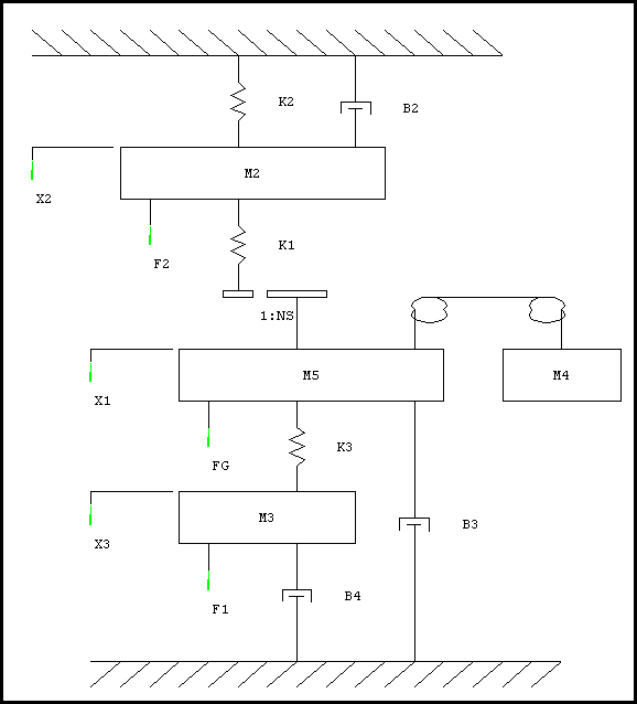
Figure 2. Tower Area Mass/Spring Diagram
First, in order to represent the strip with fixed springs and use Hooke's Law, bridle #1 and bridle #3 were considered to be at stall. As shown in Appendix D equation (D.6), the tension in the tower tension zone will only follow Hooke's Law when bridle #1 is stalled. This same idea holds true for bridle #3.
The tower carriage is counterweighted such that a downward directed force is always required to act on the carriage under all operating conditions. This was confirmed by monitoring the entry tower tensioner motor armature current and verifying that its polarity did not change during carriage acceleration or deceleration. For this reason, the portion of chain in which the jockey sprocket provides tension was not included in the model.
The accumulator was represented as a gear ratio equal to the number of strands in the tower . The masses of the accumulator rolls and strip were ignored. The effect of roll inertia on strip tension, which can be considerable during acceleration and de-acceleration, is analyzed in Appendix C.
A number of helper rolls, move the strip through the tension zone between bridle #2 and bridle #3. To keep the model simple these rolls were also ignored.
The system could then be represented by two dampers, three springs, and four masses in a linear frame of reference. The following list describes each of these elements:
|
B2 |
bridle #2 damping to ground [LB.SEC/FT] |
|
B3
|
tower carriage/counterweight damping to ground [LB.SEC/FT]
|
|
B4
|
tower tensioner-motor damping to ground [LB.SEC/FT]
|
|
K1
|
tower zone strip spring constant [LB/FT]
|
|
K2
|
bridle #2 zone spring constant [LB/FT]
|
|
K3
|
tower tensioner-motor to tower carriage spring constant [LB/FT]
|
|
M2
|
bridle #2 motor and rolls mass [SLUGS]
|
|
M3
|
tower tensioner-motor mass [SLUGS]
|
|
M4
|
tower counterweight mass [SLUGS]
|
|
M5
|
tower carriage mass [SLUGS]
|
|
Ns
|
Number of strands in the tower []
|
Letting M1=M4+M5, will leave six energy storage elements, resulting in a sixth order mechanical model.
The force and position variables shown in the Figure 2 are:
|
F1
|
tower tensioner-motor force [LB]
|
|
F2
|
bridle #2 motor force [LB]
|
|
FG
|
force on carriage due to gravity [LB]
|
|
X1
|
position of carriage [FT]
|
|
X2
|
position of bridle #2 [FT]
|
|
X3
|
position of tower tensioner-motor [FT]
|
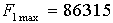
In order to approximate the value of B4, a chart recording taken during start-up was used as a reference. The chart showed approximately 10% tower tensioner-motor armature current at full carriage speed without the tower chains installed. Rated motor force can be calculated as follows:
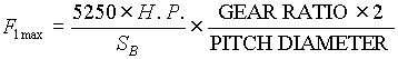
 [LB] [LB]
Full carriage speed can be calculated as follows:
 [FPM] [FPM]
B4 can then be approximated by:
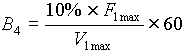
 [LB.SEC./FT] (at max speed) [LB.SEC./FT] (at max speed)
B3 was approximated to be 1/5 B4 or 2500 [lb.sec/ft]. Using 10% of total bridle #2 motor torque (15 [HP] @ 1320 [RPM]) at full speed results in B2 being approximately 10 [lb.sec/ft].
The following figure shows that at small velocities, such as those experienced near stall, the damping can be an order of magnitude higher than the value read off the linear viscous damping curve. This would depend on the magnitude of the coulomb friction in comparison to the viscous damping. From the empirical data obtained at the facility (see Chapter 2) a good approximation would be to let the viscous damping factors, calculated above, be multiplied by 10.
Figure 3. Effects of Friction on Damping Coefficients
The spring constants used in Hooke's Law for the steel strip can be calculated using the following equation:

Where:
|
E
|
Young's modulus for strip
|
|
A
|
cross sectional area of strip
|
|
L
|
length of strip
|
The cross sectional area will change with product and the length of the strip in the tower tension zone.
K3 was calculated using data from the disk spring manufacturer, Schnorr Corp. A chain to carriage connection point at each corner of the carriage contains a stack of eleven Schnorr #022-200 disk springs. Each spring deflects 5.5 mm at 165,000 Newtons of force. K3 can then be calculated as follows:
 [N/mm] [N/mm]
Converting to English units:
 [LB/FT] [LB/FT]
Carriage and counterweight masses can be obtained by dividing the weight in pounds by 32.174 (G). The motor WR2 (inertia) can be converted to a mass in a linear reference frame as follows:
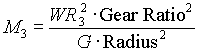
Tower tensioner-motor torque can be converted to an equivalent force by multiplying by the gear ratio and dividing by one-half the sprocket pitch diameter. Tower tensioner-motor position is the linear position of the tower tensioner-motor.
Bridle motor torque can be converted to an equivalent force by multiplying by the gear ratio and dividing by the roll radius. Bridle motor position is the linear position of the bridle motor.
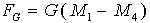
The force on the carriage due to gravity can be calculated as follows:
The following equations can then be written by summing the forces acting on each mass:
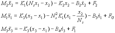
Taking the Laplace transform:
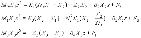
Rearranging terms and placing the equations in matrix form yields:
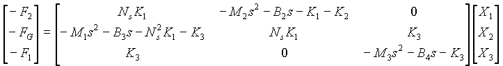
which can be written as Y = A X
Where:
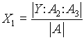 
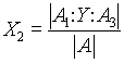 
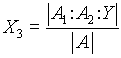 
The characteristic equation of the A matrix is given by:
And:


Where:
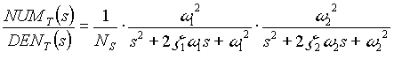
Entry Tower Torque to Tension Transfer Function
Referring to Figure 2 and using Hooke's Law, the tower zone tension T1 can be obtained using the following equation.
If bridle #1 is assumed to be of a much slower response than that of the tower tension control, F2 can be considered to be constant. Since FG is constant, the s-domain equation for T1 can be written:
Neglecting the tension offset of (F2 + FG), the transfer function can be written:
 (1.1) (1.1)
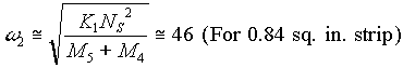
The following figure shows a Bode plot for equation (1.1) with the tower full and a strip 28 in. wide and 0.030 in. thick equivalent to a cross sectional area of 0.84 in.2.
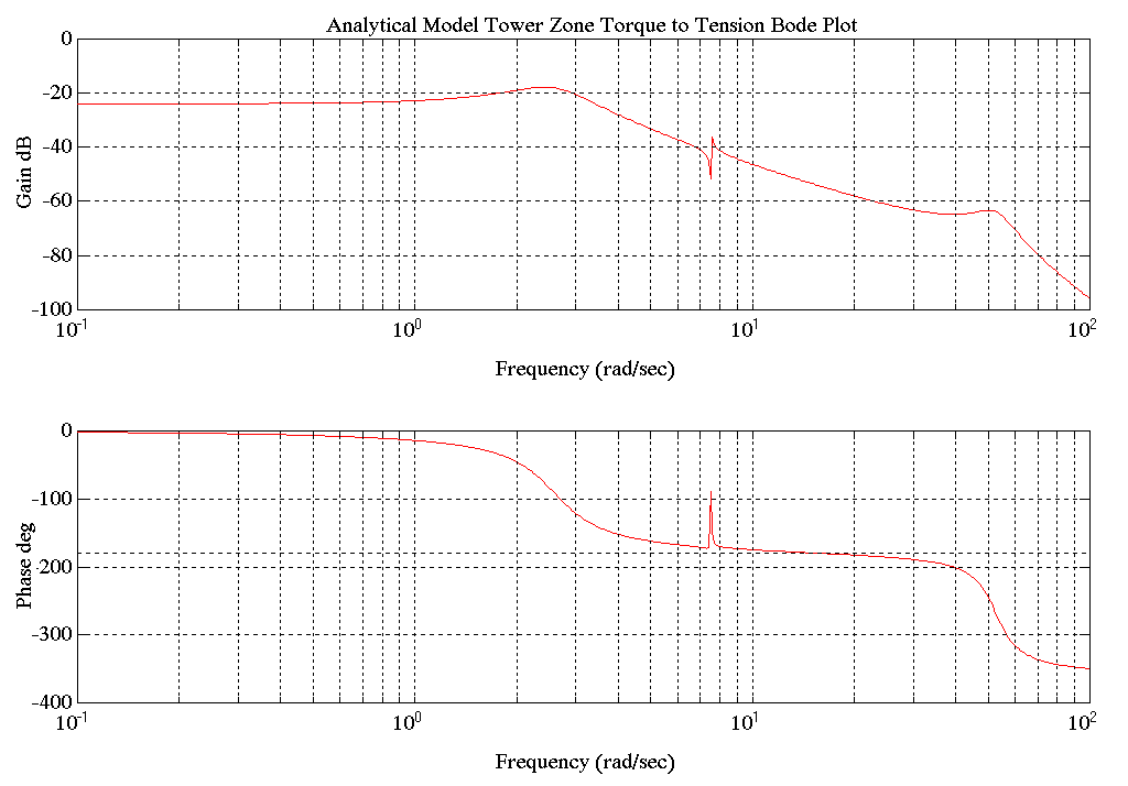
Figure 4. Bode Plot of Analytical Model Torque to Tension
Entry Tower Torque to Speed Transfer Function
Taking the derivative of the tower motor position will yield the tower motor speed:

Again, with FG and F2 constant, the transfer function can be written:
 (1.2) (1.2)
The following figure shows a Bode plot for equation (1.2) with the tower full and a strip 28 in. wide and 0.030 in. thick or a cross sectional area of 0.84 in.2.
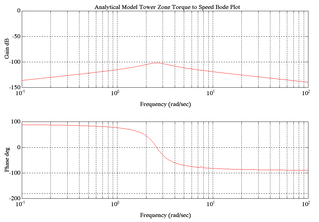
Figure 5. Bode Plot of Analytical Model Torque to Speed
CHAPTER 2
SYSTEM IDENTIFICATION MODELS
The system identification problem is to estimate a model of a system based on observed stimulus/response data. Several ways to describe a system and to estimate such descriptions exist, they can be non-parametric based, such as spectral analysis, or parametric based. Parametric based methods are based on configurations employing the autoregressive series of the form :
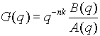
 (2.1) (2.1)
The coefficients  are the autoregression parameters. are the autoregression parameters.
The most useful and widely used parametric methods are based on variations of the following system model:
 (2.2) (2.2)
where:
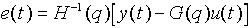
 is the measured output at time t is the measured output at time t is the known input stimulus delayed by n sample time delays that "produced" the known measured output. is the known input stimulus delayed by n sample time delays that "produced" the known measured output. represents the error between the desired output and the model output at time t represents the error between the desired output and the model output at time t- q is the delay operator (i.e

in the discrete time domain)
The objective of the system identification algorithms is to find optimum values of the parameters in A,B,C,D,F above such that the model gives outputs to the input stimulus that are an acceptable match to the measured system outputs.
This report utilized the ARX (Auto-regressive with external input) identification method described below.
arx system identification method
The ARX method, which is computationally the least complex of the parametric methods, is the most commonly used identification method. Experience has shown that the results obtained with this method are typically adequate for applications where there is a good correlation between the inputs and outputs of the system. It is also the only parametric method that lends itself to modeling of multiple-input multiple-output (MIMO) systems.
This model is described by:
 (2.3) (2.3)
Thus the ARX structure is the same as (2.2) where nc=nd=nf=0.
To find the parameters that yield the best fit between the model and experimental outputs the following algorithm is implemented:
let:
we can then express the error in 2.3 as:
 (2.4) (2.4)
(see [1] pp. 1-10 : 1-12 for detailed derivation of (2.4))
These errors are, for given data y and u at time t, functions of G and H. These in turn are parametrized by the polynomials in (2.3). To identify these parameters we minimize
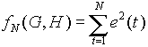 (2.5) (2.5)
The method that is used by the MATLAB system identification toolbox to find the set of coefficients (parameters) for A and B in G and H that minimize the error function (2.5) is the Maximum Likelihood Method (see [2] Ch. 7 for description).
OBTAINING stimulus/response data. THE DATA collection software
The following figure shows a block diagram for the software installed in the entry and delivery tower intermediate loop regulator tasks.
The forcing function generator, provides the stimulus to the system by generating the value of the Boolean variable sid_ff_on@. The variable sid_ff_on@ changes state each time the system identification scan counter is equal to a scan count which is read from a table of values which define the forcing function transitions. The variable sid_ff_on@ will switch the value of sid_ff_amp% into the summer, effectively adding the value of sid_ff_amp% to the armature current reference. A limit block insures that current limit is not exceeded during the system identification process.
In order to obtain the best possible correlation between the stimulus and response, sid_cur_ref_1% was forced during the system identification process.
The following variables are sampled every 0.022 [sec] for up to three minutes:
|
sid_cur_ref_1%
|
current reference w/o forcing function [4095=1.75 Ia]
|
|
sid_ff%
|
forcing function [4095=1.75 Ia]
|
|
MAJOR_I_FDBK%
|
current feedback [4095=1.75 Ia]
|
|
tach_fdbk%
|
scaled resolver feedback [4095=Sb]
|
|
FORCE_FDBK%
|
tension fdbk [4095=MAX TENSION*10000/T_FDBK_CALIB% LB]
|
The sampled data is then stored in SID_DATA%
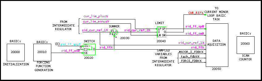
Figure 6. System Identification Data Collection Program
A new program was added to the tower drops, to print the data in the SID_DATA% array to the serial port. The Drive Vendor Service Department's Log Data utility, running on an IBM compatible, was then used to capture the data and write it to a 3 1/2" floppy disk. The entry tower intermediate loop is a 10 [ms] task. This required that the Distributed Control System (DCS) processor, in the entry tower, be replaced with a faster processor when the system identification code was added. Also, the Common Memory board on both towers at the facility were upgraded to provide the increased memory required to store the system identification sampled data.
results
After the installation of the hardware and software at the entry and delivery towers, data was collected from both towers under stall and run operating conditions. ARX Models of the system were then obtained for the various operating conditions using the MATLAB System Identification Toolbox and proprietary script files. The MATLAB script files were written to convert the ARX polynomial model description into z-domain transfer function descriptions, and from the z-domain into the s-domain with a pre warped bi-linear transformation (warped about 2.5 [rad/sec]), from which the poles and zeroes of the system at the given operating condition were able to be extracted. Bode plots were also generated from the obtained s-domain transfer functions.
As explained previously, data was obtained for both motor shaft speed and strip tension. The results for the data taken at the entry and delivery towers are presented in two sets for each tower. The first set refers to the transfer function between current reference (torque) and strip tension. The second set between current reference and motor shaft speed. Each set contains one or more of the following plots.
- The input stimulus and the measured response.
x-axis => [Sample No.] (sample rate of .022 [sec])
y-axis => [lbf]
- The measured and ARX model responses to the above input stimulus.
x-axis => [Sample No.] (sample rate of .022 [sec])
y-axis => De-trended [lbf]
- Bode (Magnitude and Phase).
ARX model parameters and the obtained pole zero locations for each model are presented in Appendix E.
Entry Tower
Data (filename in parenthesis) was obtained for the following system operating conditions:
- Condition A) (SPE1.MAT) Line in stalled condition, brakes locked on bridle #1 and bridle #3.
Strip = .030 [in] x 28 [in] (.84 [sq. in.])
- Condition B) (SPE2.MAT) Line running. Tower began emptying @ sample no. 1850.
Strip = .046 [in] x 33.75 [in] (1.55 [sq. in.])
- Condition C) (SPE5.MAT) Line running. Tower 30% full.
Strip = .030 [in] x 39 [in] (1.17 [sq. in.])
- Condition D) (SPE6.MAT) Line running. Tower full
Strip = .028 [in] x 40 [in] (1.12 [sq. in.])
Entry Tower Torque to Tension Transfer Function
Condition A) This operating condition is closest to that which satisfies the assumptions that were made in the derivation of the analytical model described in Chapter 1. Since the line was stopped and the brakes were engaged on bridle #1 and bridle #3, the entry tower was effectively isolated from outside disturbances.

Figure 7. S.P. Stimulus/Response SPE1.MAT Tension
The following plot shows the de-trended measured and model responses (de-trended here refers to the process of removing the average value offset in the data). The model is stimulated with the same data used to stimulate the process when the input/output data was taken.
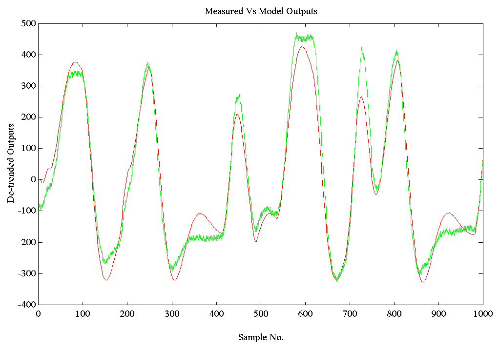
Figure 8. Output Comparison SPE1.MAT Tension
After the ARX polynomial model of the plant has been derived, an s-domain transfer function is obtained as described previously. From this s-domain transfer function a bode plot is generated, and is presented below.

Figure 9. Bode Plot SPE1.MAT Tension
It was known that the entry tower employed a 2nd order anti-aliasing filter set at 20 [rad/sec] to filter the tension feedback. This did not appear in the above Bode plot, a more accurate system identification method was used to pick out this pole pair. This is known as the IV (Instrumental Variable) method .(see [1] 2-48 to 2-53). While this method is more difficult to work with, the final result is typically better than that obtained with the ARX method.
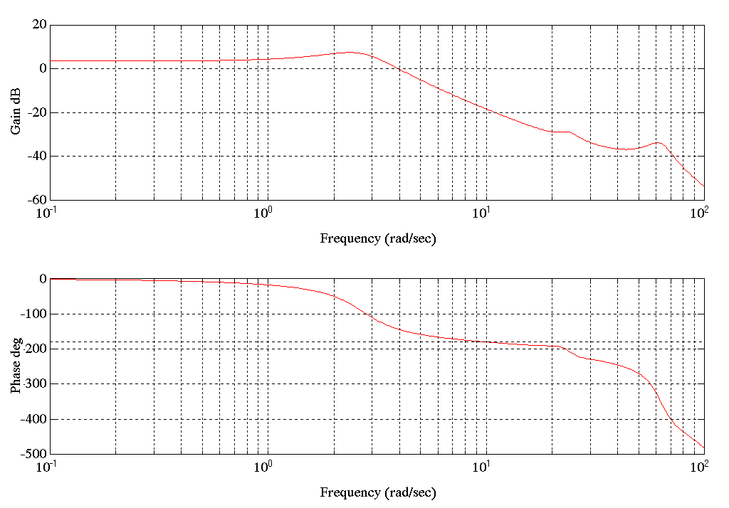
Figure10. Bode Plot SPE1.MAT Tension (Using the IV Method)
Condition B) The results of this operating condition represent a "snapshot "of the model of the entry tower when operating dynamically with heavy strip. It was observed that the tower broke into a 2-3 [rad/sec] oscillation when the tower started emptying, while the stimulus supplied by the forcing function used to obtain the SID data was being applied. This was immediately registered as a 2-3 [rad/sec] oscillation in the strip tension. This did not occur when the SID program was not running. This indicated that the SID forcing function excited the 2-3 [rad/sec] resonant mode in the tower. It was also observed that when the resonance occurred the chains in the tower began to sway at the same frequency. The following plot clearly demonstrates this phenomena. The tower began emptying at sample No.1850
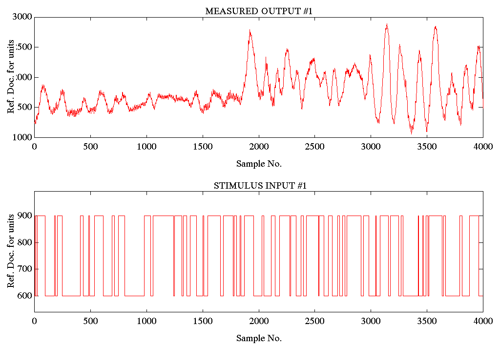
Figure 11. S.P. Stimulus/Response SPE2 Tension
An ARX model was obtained for the first 1000 samples (before the tower began emptying) above. Following is a plot of the actual Vs model outputs for that range.
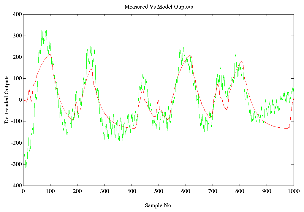
Figure 12. Output Comparison SPE2.MAT Tension
Following is the Bode Plot for the above ARX plant model. This can be considered a good snapshot of the entry tower transfer function frequency response when running heavy strip with the tower full.
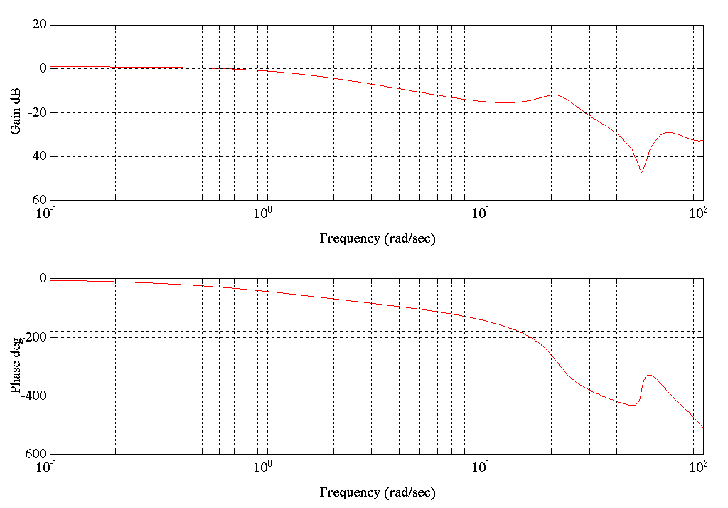
Figure 13. Bode Plot SPE2.MAT Tension
When the product was not being fed into the tower, such as is the case when the tower is emptying, the 2-3 [rad/sec] tower resonance was excited by the forcing function disturbance introduced into the control loop by the SID data collection program. When this occurred there was poor correlation between the input stimulus and the tension feedback. Consequently, the ARX model for that set of data was not a very good approximation of the plant.
Condition C) This set of results reflect the dynamic behavior of the entry tower when nearly empty. This provides a basis for comparing the entry tower to the delivery tower which mainly operates in an empty condition. Following is the Bode plot for the derived ARX model.
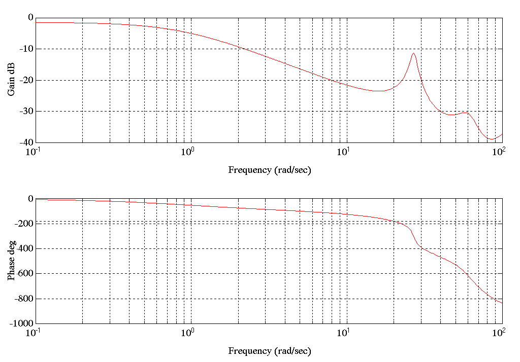
Figure 14. Bode Plot SPE5.MAT Tension
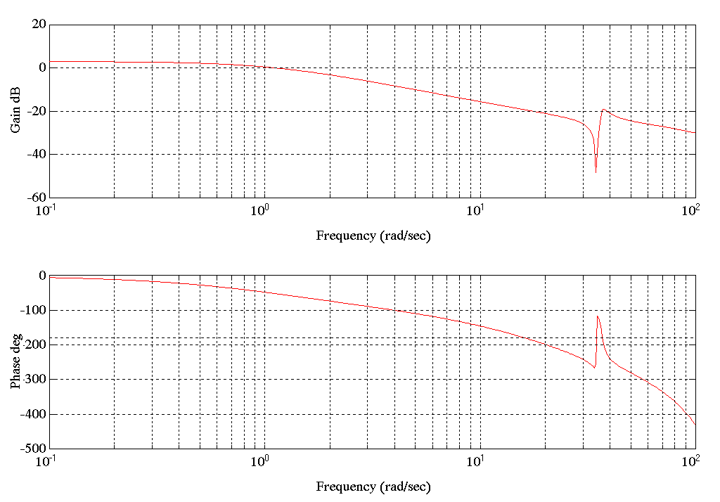
Figure 15. Bode Plot of SPE6.MAT Tension
Condition D). The Bode Plot above (SPE6.MAT) is of the plant with a full entry tower and a lighter strip.
Entry Tower Torque to Speed Transfer Function
The following set of results are for the same set of data presented in the previous section and they follow a similar format, with the exception that stimulus response plots are not presented. (They are the same stimulus sets as above)
Condition A) The Torque to Speed model for this operating condition shows clearly the 2-3 [rad/sec] resonance in the tower. Following are the output comparison and Bode plots for this configuration.

Figure 16. Output Comparison SPE1.MAT Speed

Figure 17. Bode Plot SPE1.MAT Speed
Condition B) Following is the Bode Plot for SPE2.MAT
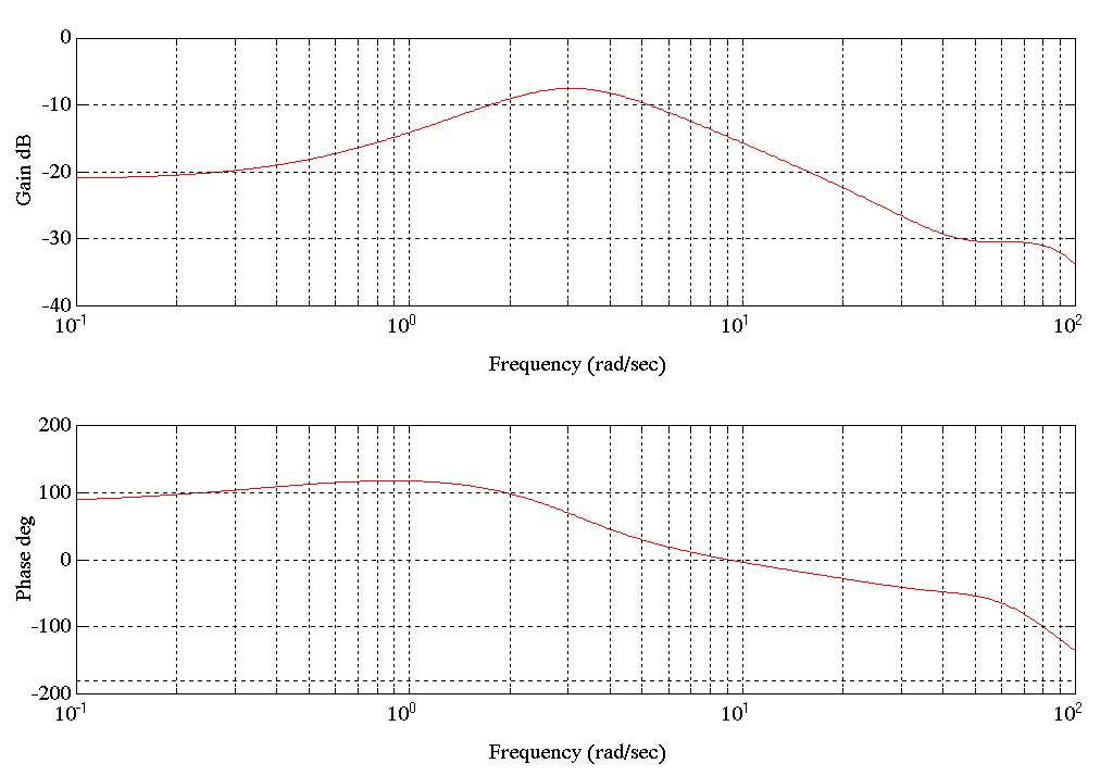
Figure 18. Bode Plot SPE2.MAT Speed
Condition C) The following Bode Plot shows that even with the tower almost empty the resonance is still very apparent.
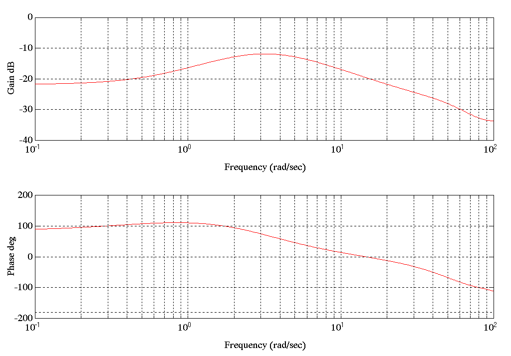
Figure 19. Bode Plot SPE5.MAT Speed
Condition D) The Bode Plot for SPE6.MAT (speed) was identical to SPE2.MAT and SPE5.MAT.
Delivery Tower
An analysis similar to that performed on the entry tower was performed on the delivery tower.
Data (filename in parenthesis) was obtained for the following delivery tower operating conditions:
- Condition A) (SPD1.MAT) Line in stalled condition. Tower 30% full.
Strip = .030 [in] x 38 [in] (1.14 [sq. in.])
- Condition B) (SPD3.MAT) Line running. Tower Empty.
Strip = .036 [in] x 36 [in] (1.30 [sq. in.])
Delivery Tower Torque to Tension Transfer Function
Condition A) As was the case in the entry tower, the ARX model produced for this configuration is most similar to the analytical model. Following are the plots of 1) comparison of actual and model outputs and 2) Bode for Condition A.
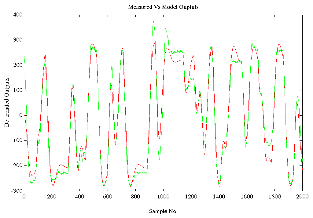
Figure 20. Output Comparison SPD1.MAT Tension
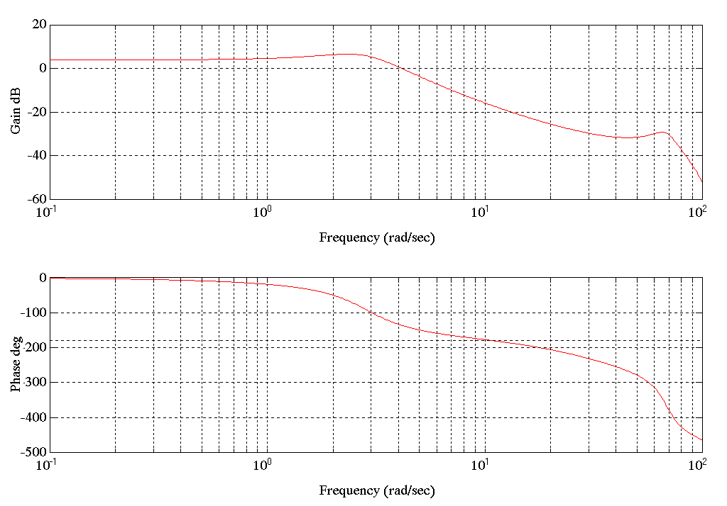
Figure 21. Bode Plot SPD1.MAT Tension
The Bode plot for SPD1.MAT has a very well damped resonance at approximately 2-3 [rad/sec]. This is to be expected in so far as the entry and delivery towers have approximately the same mechanical configuration between the motor and the carriage.
For Condition B) This set is included to provide insight into the frequency response of the delivery tower with product moving through it. Note that there is a 2-3 [rad/sec] oscillation in the data that was not picked up by the system identification method.
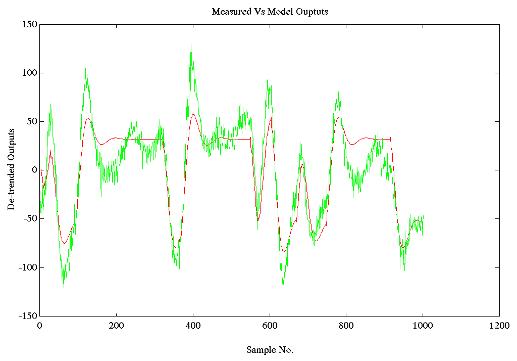
Figure 22. Output Comparison SPD3.MAT Tension
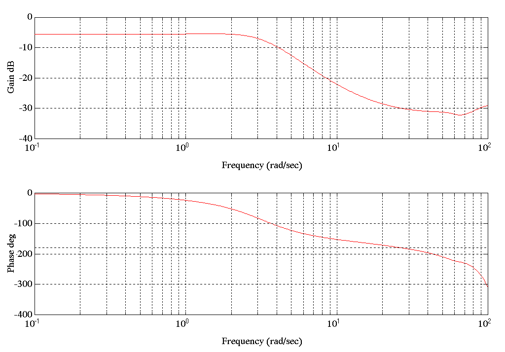
Figure 23. Bode Plot SPD3.MAT Tension
Delivery Tower Torque to Speed Transfer Function
Condition A) The Torque to Speed transfer functions for the delivery tower also exhibit the 2-3 [rad/sec] resonance seen in the entry tower. This is because of the similar coupling configurations used in both towers to connect the Carriage Drive Motor to the Carriage. From this it can be deduced with a high degree of certainty that the mass-spring resonance of the mechanical system comprising the motor gear-box, chains, carriage and counter-weights used in both towers is around 2-3 [rad/sec]. Following is the Bode Plot of the ARX model for Condition A.
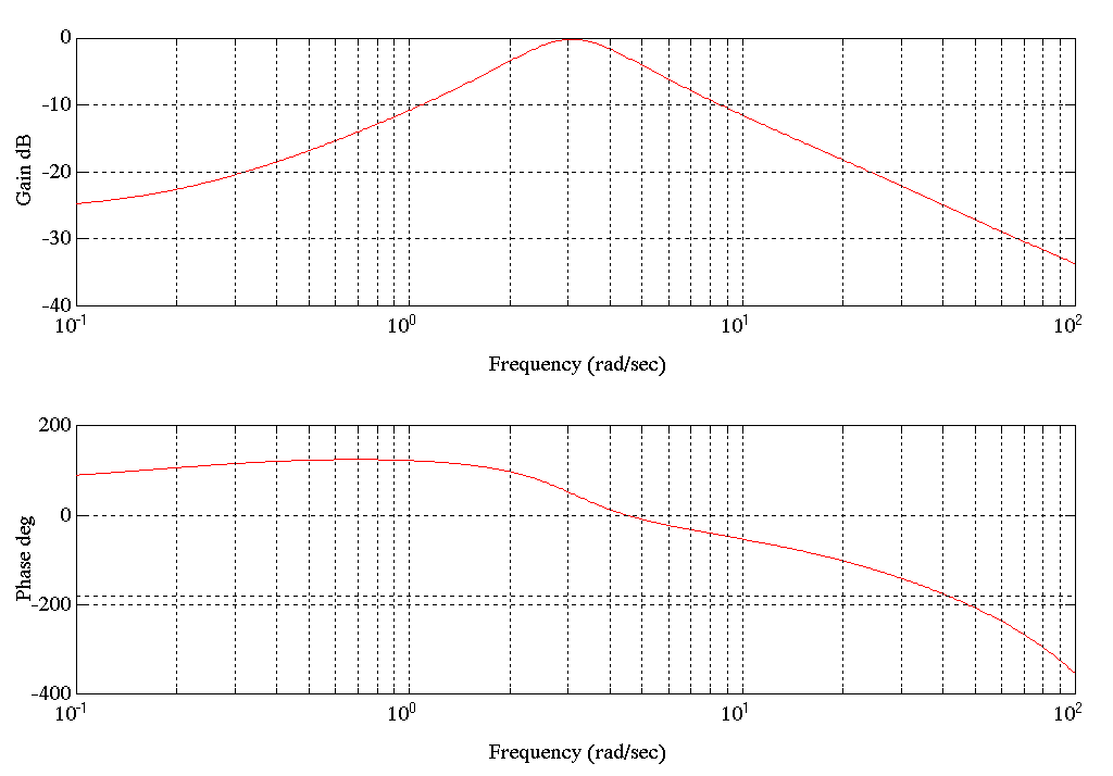
Figure 24. Bode Plot SPD1.MAT Speed
Condition B.) In this configuration we see a similar resonance to that observed above. Following is a Bode Plot of the ARX model derived for this configuration.
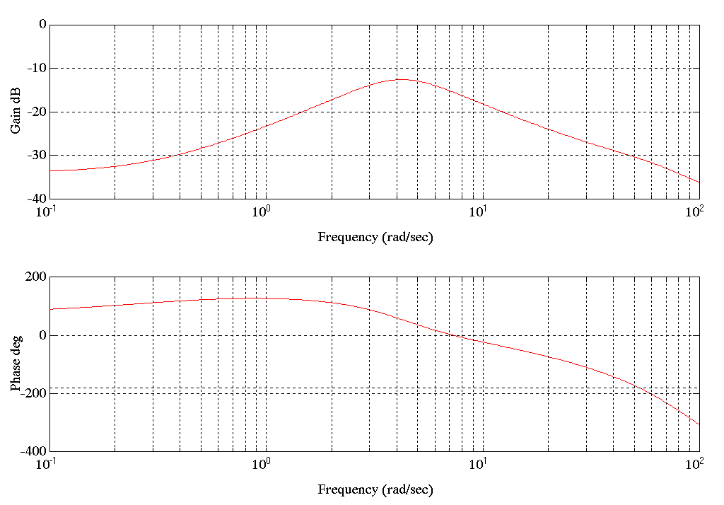
Figure 25. Bode Plot SPD3.MAT Speed
CHAPTER 3
FINAL TOWER MECHANICAL MODEL
The analytical and empirical entry tower models derived in chapters 1 and 2 both exhibit similar resonant frequencies. The low frequency resonance, at approximately 2-3 [rad/sec], is a major contributor to the instabilities observed during commissioning.
Figure 4. shows the bode plot for the analytical transfer function from entry tower motor torque to strip tension. The high frequency resonance is directly related to the strip spring constant and does not significantly contribute to the stability problems observed during commissioning. The resonance will move out with a higher strip spring constant, and in with a lower strip spring constant. The 2-3 [rad/sec] resonance is directly related to the chain/carriage attachment spring. The center frequency pole/zero pairs are a result of the mass/spring system for bridle #2.
The empirical transfer function corresponding to the analytical transfer function of Figure 4. is shown in Figure 9. The frequencies of resonance are the same but two differences are evident.
The first difference is seen as a gain offset of 28 [dB] for the motor torque to strip tension transfer function. This difference is due to the units used in each transfer function. This factor is equivalent to multiplying CTF (see equation (3.1)) by TTC (see equation (3.2)). The analytical bode magnitude plot is gain in pounds strip tension per pound motor force. The empirical bode magnitude plot is gain in counts of strip tension per count of motor armature current.
The second difference is a lack of any discernible bridle #2 dynamics in the empirical model. While the approximations of damping constant for the tower motor and carriage in the analytical model appeared to be valid, the empirical model suggests the damping constant for bridle #2 is much higher at stall.
Figure 12. shows the bode plot for the empirical transfer function from entry tower motor torque to strip tension while the line is running and the tower is full of relatively heavy product. The conditions for Figure 13. are similar to Figure 12 except with a slightly lighter product and the tower 30% full. The conditions for Figure 14 are similar to Figure 13 except with a lighter product.
Figure 5. shows the bode plot for the analytical transfer function from entry tower motor torque to motor speed. Here again the second order lag at 2-3 [rad/sec] is evident. The low frequency asymptote has a +1 slope, corresponding to an impedance dominated by the chain/carriage connection spring at low frequencies. The high frequency asymptote has a -1 slope, corresponding to an impedance dominated by the motor mass.
The empirical transfer function corresponding to the analytical transfer function of Figure 5. is shown in Figure 16.
Again a gain offset of approximately 107 [dB] for the motor torque to motor speed transfer function is evident. This factor is equivalent to multiplying CTF (see equation (3.1)) by STC (see equation (3.3)). The analytical bode magnitude plot is gain in [feet/sec] carriage speed per pound motor force. The empirical bode magnitude plot (after de-trending) is gain in counts of motor speed per count of motor armature current.
The conditions for Figures 17., 18. are similar to 16. with the line running. The most significant feature of these plots is the increase in damping.
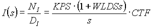
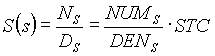
Based on these observations, the model used for the regulator analysis is a combination of both the analytical and empirical models and consists of two transfer functions, torque to tension and torque to speed. The low frequency asymptotes of the transfer functions are taken from the analytical model and are calculated from equation (1.1) and (1.2) as follows:
 (3.0a) (3.0a)
 (3.0b) (3.0b)
The resonant frequency characteristics of the transfer functions are taken from the empirical model (SPE1.MAT) and are simplified to two complex pole pairs. The first complex pair is set at 2.6 [rad/sec] with a damping factor (z1) of 0.34 with bridle #1 stalled. This complex pair represents the resonance dominated by the motor mass and the chain/carriage connection spring. The undamped natural frequency can be approximated as follows:
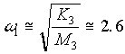 [rad/sec] [rad/sec]
In Figure 10 the effect of the 2nd order anti-aliasing filter in the tension feedback can be seen. This pole pair was set to roll off at approximately 20 [rad/sec] with a z of 0.75. This represents the second most dominant resonant pole pair in the current major with speed intermediate loop control configuration presently implemented in the entry tower DCS controller.
A third complex pole pair is at approx. 46 [rad/sec] with a damping factor (z2) of 0.25 representing the tower zone strip resonance. This lag was included in the model since it affects phase margin. This frequency can be approximated by:
The final tower mechanical model is comprised of the first and third pole pairs from above. The second pole pair (or the effect of the tension feedback filter) was included in the model of the Tension Major with Speed Intermediate control configuration. This was the only configuration for which the filter was set at the 20 [rad/sec] cutoff freq.
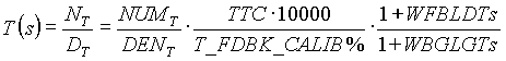
Three conversion factors CTF (counts to carriage force), TTC (tension to counts) and STC (carriage speed to counts) are included in the model to convert between engineering units and counts. These factors are calculated as follows
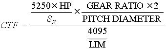 [lb/count] (3.1) [lb/count] (3.1)
For the entry tower CTF=37
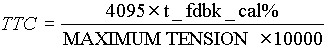 [counts/lb] (3.2) [counts/lb] (3.2)
For the entry tower TTC=0.69
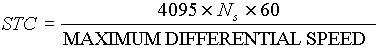 [counts-sec/ft] (3.3) [counts-sec/ft] (3.3)
For the entry tower STC=5850
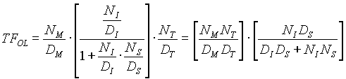
The following block diagram shows the model used for regulator analysis in Chapter 4.
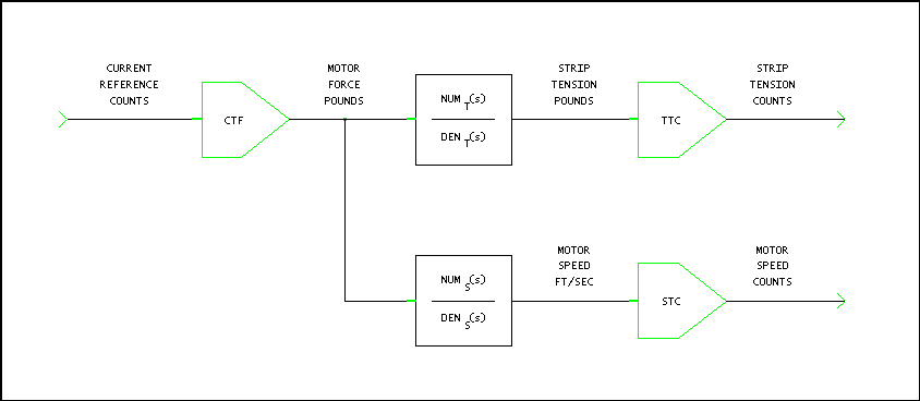
Figure 26. Final Plant Model for Regulator Analysis
Where from the Figure 26 above we have:
For the torque to speed transfer function:
 (3.4) (3.4)
For the torque to tension transfer function:
 (3.5) (3.5)
The speed loop is modeled with only the dominant complex pair at 2.6 [rad/sec]. This was done based on the responses of both the analytical and empirical models, where the effect of the high frequency resonant pole pair was observed to be negligible (ref . Figures 5 and 16).
Following are the bode plots of the final mechanical models. Note that these Bode plots are very similar to the analytical and empirical (in stall) Bode plots (ref. Figures 4 and 5, 9 and 16)
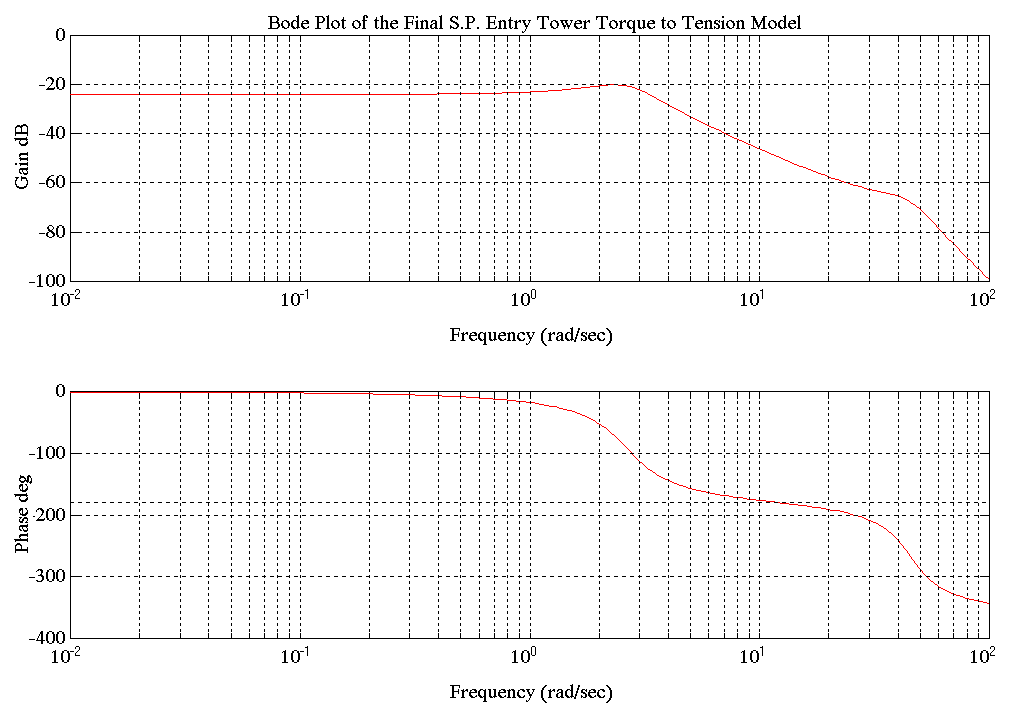
Figure 27. Bode Plot of Final Torque to Tension Model
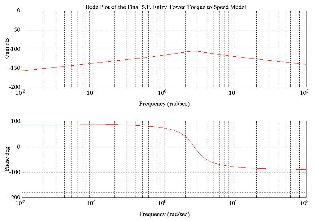
Figure 28. Bode Plot of Final Torque to Speed Mechanical Model
This concludes the section on the final model derivation.
CHAPTER 4
MODEL WITH DCS REGULATION
Each accumulator tower has four regulating loops implemented in a proprietary DCS control block language. These loops are; tension, speed, current major, and current minor.
The current minor loop crossover in continuous conduction is approximately 150 [rad/sec] and is not included in the analysis since it is approximately a factor of 100 greater than the tension loop crossover.
The DCS controller is a digital regulating system which uses digitally sampled feedback. The sample rate for the tension and speed loops is 45 [samples/sec]. The sample rate for the current major loop with the speed intermediate loop is also 45 [samples/sec]. The sample rate for the current major loop without the speed intermediate loop is 90 [samples/sec]. Since the sample rates were sufficiently high, compared to the corresponding regulating loop bandwidth, the digital nature of the control was ignored and the analysis was done completely in the s-domain.
Later in this chapter, the tension, speed, and current major loops are configured and tuned several different ways. This reflects the various tunings encountered during the commissioning process. The regulator configuration is represented in block diagram form. The values of the tuning parameters for the different regulators can be found in Appendix B.
The analysis does not include feed-forward signals such as WR2 compensation. Since the feed-forward signals are derived from the tension and speed references, the analysis assumes the references are constant.
Tension Feedback Hardware Filters
There are two hardware filters acting on the entry and delivery tower tension feedback signals. The first is a first order hardware filter implemented on a custom card. The second, a second order Bessel filter is located on the DCS analog input card.
The first order hardware filter was not included in the analysis because the dampening pots were set to zero. At zero there is no lead or lag introduced into the feedback. The second filter was set at 150 [rad/sec] for all except one of the following regulator configurations. The exception was the present configuration for the entry tower. In this case the filter is set at 20 [rad/sec] and would affect the performance of the Tension Major with Current Intermediate control configuration. It was therefore included in the analysis of this configuration.
Entry Tower Tension Regulation
With Speed Intermediate Loop
The following simplified block diagram shows the entry tower regulator as it was configured on the day of data collection. For the analysis, the blocks were placed in one of four groups, indicated by the dashed boxes.
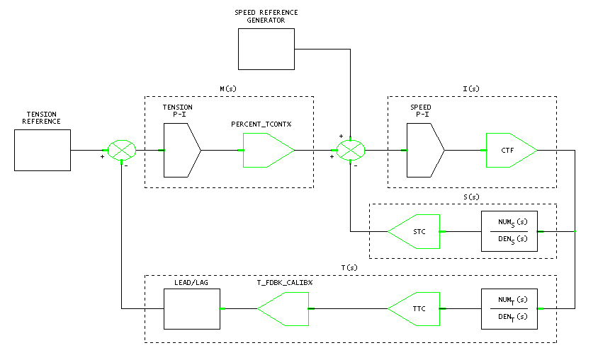
Figure 29. Entry Tower Tension Major Loop with Speed Intermediate Loop
For the regulator derivations the following plant models apply:
(speed) (3.4)
 (tension) (3.5) (tension) (3.5)
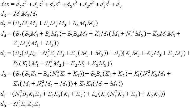
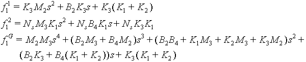
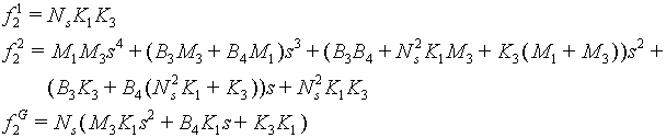
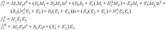
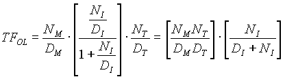
The open loop transfer function was then simplified as follows:
 (4.1) (4.1)
 (4.2) (4.2)
 (4.3) (4.3)
 (4.4) (4.4)
 (4.5) (4.5)
The following are Bode plots for these transfer functions:
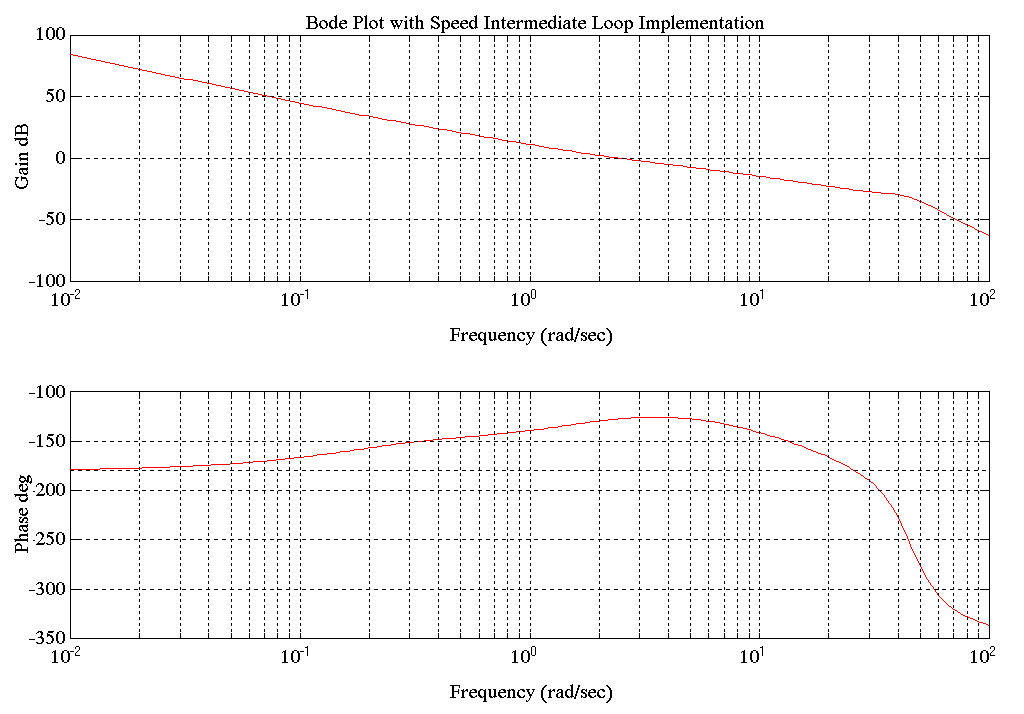
Figure 30. Entry Tower Tension Major Loop with Speed Intermediate Loop Bode Plot

Figure 31. Entry Tower Speed Intermediate Loop Bode Plot
With Current Intermediate Loop
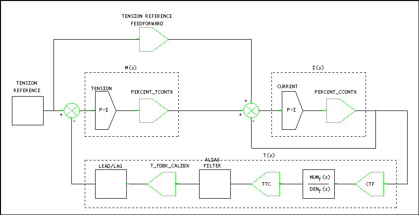
Figure 32. Entry Tower Tension Major Loop with Current Intermediate Loop Block
 (4.6) (4.6)
 (4.7) (4.7)
 (4.8) (4.8)
 (4.9) (4.9)
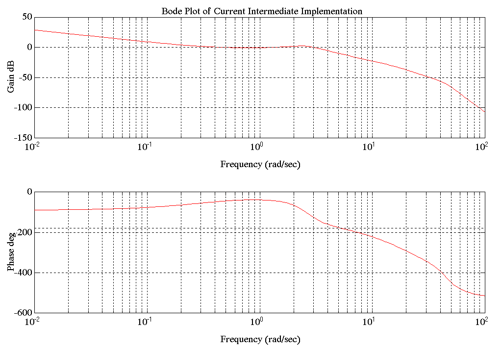
Figure 33. Entry Tower Tension Major Loop with Current Intermediate Loop Bode Plot
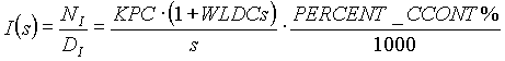
Entry Tower Current Regulation
With Speed Intermediate Loop
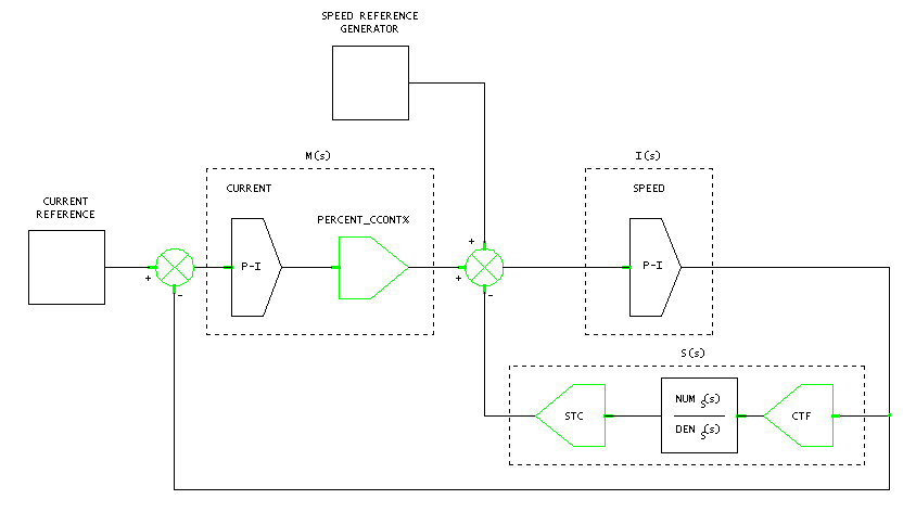
Figure 34. Entry Tower Current Major Loop with Speed Intermediate Loop Block Diagram
 (4.10) (4.10)
 (4.11) (4.11)
 (4.12) (4.12)
 (4.13) (4.13)
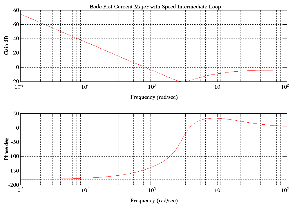
Figure 35. S.P. Entry Tower Current Major Loop with Speed Intermediate Loop Bode Plot
Without Speed Intermediate Loop
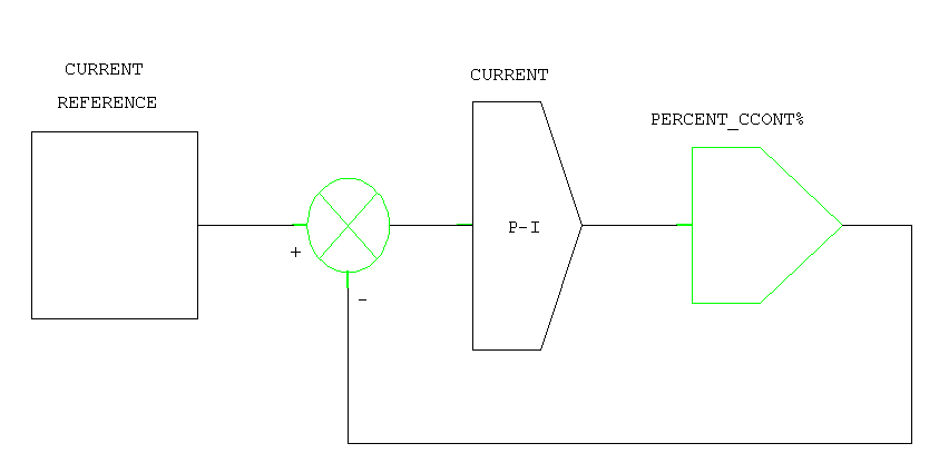
Figure 36. Entry Tower Current Major without Speed Intermediate Loop Block
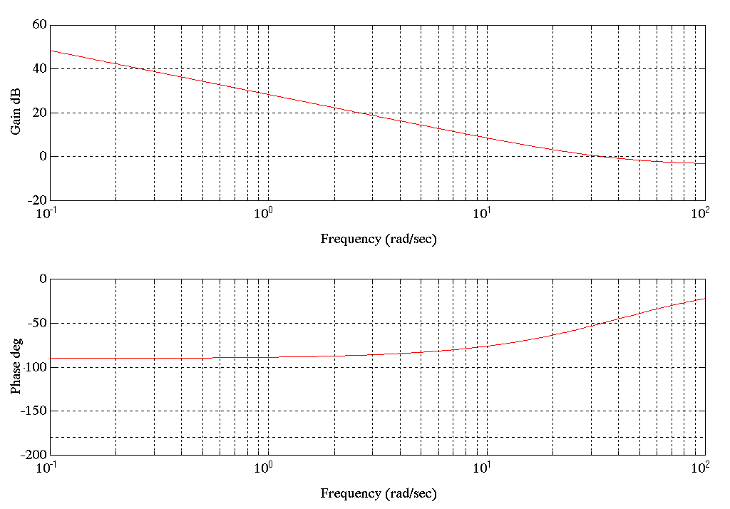
Figure 37. Entry Tower Current Major Loop w/o Speed Intermediate Loop Bode Plot
Delivery Tower Tension Regulation
Only a Bode plot is included, the architecture is the same as the entry tower.
With Speed Intermediate Loop
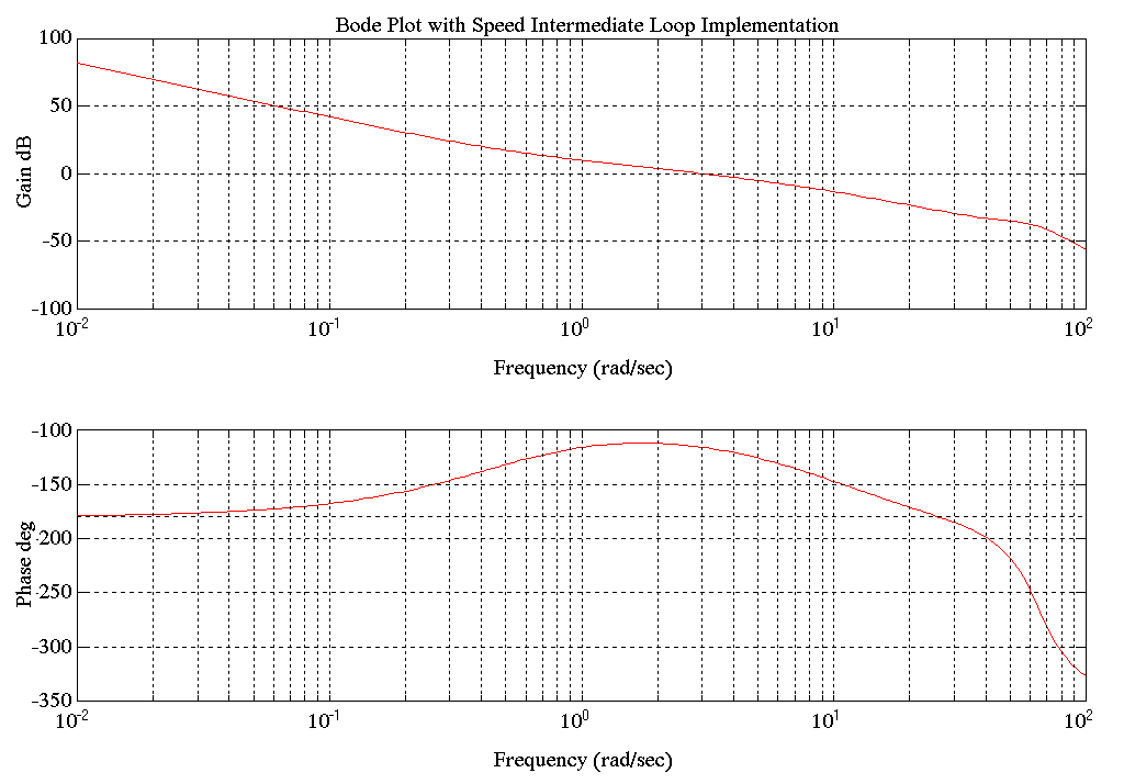
Figure 38. Delivery Tower Tension Major Loop With Speed Intermediate Loop Bode Plot
Delivery Tower Current Regulation
Only a Bode plot is included, the architecture is the same as the entry tower.
With Speed Intermediate Loop
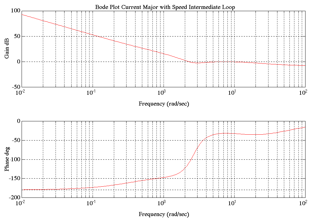
Figure 39. Delivery Tower Current Major Loop With Speed Intermediate Loop Bode Plot
CHAPTER 5
OBSERVATIONS AND CONCLUSIONS
Observations
1) The analytical results and empirical data for the entry tower clearly show a resonance of 2-3 [rad/sec]. This resonance was also observed in the empirical data for the delivery tower, but with more damping.
2) The entry tower was observed to go unstable at the same frequency. This occurred (during the data collection) when the #1 bridle was stopped and the tower began emptying. This can be verified in Figure 10.
3) 2-3 [rad/sec] resonance was considerably more damped when the line was running. This can be verified in Figure 9 (stall) and Figure 12,13 and 14 (running).
4) The chains that coupled the motor sprocket to the carriage springs were noticed to sway at approximately 2-3 [rad/sec] when the instability was observed. Also when this occurred the resulting ARX system model was poor. This indicated that the resonance in the tension behaved as if it was the result of an external noise source (such as the chains swaying and pulling on the carriage). This led to a poor correlation between the input stimulus and the output response.
5) During line run conditions many resonances of varying frequency and damping were observed between 20-100 [rad/sec]. These dynamics are similar to those present in the analytical model that relate to bridle #2 dynamics. They may be attributed to the dynamics of process line tension zones and speed regulators adjacent to the entry tower.
6) Between 12/4/92 and 1/12/93, tension loop gain of #2 bridle was decreased by a factor of 3. Bridle #3 was also detuned. With this softened #2 and #3 bridle tension control we did not observe any significant change in system behavior with strip gauges below .048" that were run while we were taking data. It was noted in other reports, that were made when the #2 and #3 bridle tension control was stiffer, that the system was very sensitive to strip gauge over .050" (ref. memo 12/8/92 by D. J. Unite)
7) Observations from the Regulation Bode plots.
| |
Regulation
|
w co
|
Phase Margin
|
Stability
|
Type
|
|
A
|
Entry Tower Ten. Maj. w. Spd. Int.
|
2.53
|
53.8
|
good
|
2
|
|
B
|
Entry Tower Ten. Maj. w. Curr. Int.
|
0.25
|
64
|
fair
|
1
|
|
C
|
Entry Tower Curr. Maj. w. Spd. Int.
|
0.73
|
34
|
poor
|
2
|
|
D
|
Delivery Tower Ten w. Spd. Int.
|
3.0
|
64
|
good
|
2
|
|
E
|
Delivery Tower Curr. Maj. w. Spd. Int.
|
2.3
|
71
|
fair
|
2
|
|
F
|
Entry Tower Curr. Maj. w/o Spd. Int.
|
32
|
130
|
excellent
|
1
|
A & D) This can be seen to be type 2 from the denominator of equation 4.5. Two s's can be factored out of DM , DI, and NS .
B) This can be seen to be type 1 from the denominator of equation 4.9. One s can be factored out of DM .
C & E) This can be seen to be type 2 from the denominator of equation 4.13. Two s's can be factored out of DM , DI, and NS .
Another interesting observation is that the open-loop transfer functions of the Current Major Loop with Speed Intermediate control configurations had the plant denominator polynomial in the numerator. This led to the 2-3 [rad/sec] pole pair appearing as an under-damped lead rather than a lag in the open-loop transfer function.
Conclusions
Very often, the first concern, when modeling the mechanics of a process line tension regulator, is the resonance that will be present due to the spring-like nature of the strip material. In Chapter 1 the analytical model contained a strip resonant frequency equal to approximately 50 [rad/sec] with the tower nearly full and a strip cross sectional area of 0.84 [in2]. Although this resonant frequency could be as low as 24 [rad/sec] with the lightest strip, it was clear that dynamics other than the strip resonance were lower in frequency and would therefore be more dominant.
The analysis shows clearly that the resonance at 2-3 [rad/sec] is a problem. The natural frequency of the tower chains had also been observed to be approximately the same frequency. Accumulator tower chains have been shown to have a natural frequency of approximately 1.8-2.2 [rad/sec] ([6] pp.4) at other sites. The inability of the regulation schemes to control this resonance, which occurs close to the crossover of the tension loops, may be explained by the chains swaying 180 degrees out of phase with the response of the regulator to the tension transients caused by the swaying of the chains. Under this assumption, the energy supplied by the regulator to suppress the resonance would be fed into the swaying of the chains. Had this non-linear aspect of the system been included in the analytical model it may have been more readily visible during the analysis.
An important phenomena that is somewhat hard to explain, is the change in the low frequency under-damped resonance to that of an over-damped response when changing from the stalled condition of Figure 9 to the running condition of Figure's 12, 13 and 14 (this can be seen in the various empirical model pole positions in Appendix E). From the derivation shown in Appendix D, we see that the effect of bridle #1 introducing strip into the tower tension zone changes the transfer function of carriage speed to strip tension from a pure integration to a first order lag (ref. D.5). However, even with bridle #1 at full speed the transfer function around the frequency band of interest is largely unaffected. We believe that by releasing the brake on bridle #1 and the brakes on sections downstream of bridle #2, a "softening" of the system is introduced, that both reduces the low frequency resonance and provides damping. This is analogous to allowing movement of the ground plane shown in the top of Figure 2. The concept of a soft lead section providing damping is not a new one (ref. [5] p.2) and could explain a number of observations made during commissioning. Stopping bridle #1, as is the case when the entry tower is raising, will stiffen the system. Heavier strip and/or more responsive adjacent section regulation will also stiffen the system. De-tuning adjacent tension zones will "soften" the system and, as observed, reduce the sensitivity of the system to variations in strip gauges. Any stiffening of the system, as observed empirically, will tend to peak the 2-3 [rad/sec]resonance.
If the mechanical system and all adjacent sections are relatively stiff, the only spring that must be considered is the strip. With a material such as steel, this spring constant is extremely high and the gain in the transfer function from torque to speed is negligible at and below the tension crossover frequency. This would allow a simplification where-in this block may be eliminated entirely. This is equivalent to opening the speed loop. Further, if the line speed is small compared to the length of material in the tension zone, the system model in a stall condition is a good approximation of the line in a run condition (see Appendix D). This is the approach taken during the original design of the tower tension regulator. However, since the tower has a low frequency resonance in the 2-3 [rad/sec] area, this simplification cannot be made.
Analysis of the Tension Major Loop with Speed Intermediate control showed that the plant poles are canceled out of the open loop transfer function. This is true under the assumption that the speed and tension plant transfer function denominators are similar to each other (see equation 4.5). This implies that the speed intermediate loop provides very good damping of the plant resonances in the open loop transfer function.
The Tension Major Loop with Current Intermediate control was found to be far more sensitive to changes in the damping of the plants resonances. It is a type 1 system, the other tension/current major loop control configurations were found to be type 2.
The Current Major Loop with Speed Intermediate control Bode plot did not look at all as expected. The 2-3 [rad/sec] plant resonance, as observed above, places an unexpected 2nd order under-damped lead at a critical frequency of the open loop transfer function. In this configuration a lowering of the proportional gain or the lead frequency of the current major loop regulator will induce instability rather than suppress it. This would make the regulator hard to tune if the on-site engineer assumed that lowering the gain and the Wldc values would reduce instability. (see Figures 34 and 37). This may explain why, during commissioning, the Current Major Loop was uncharacteristically found to be marginally stable.
The Current Major Loop without Speed Intermediate control does not have any plant dynamics in the open loop transfer function. This would explain why it was found to be more stable and easier to tune than the previous configuration. One important drawback to the use of this configuration is the loss of speed limiting during a strip break. A comparison of carriage speed to entry and process strip speed provides strip break detection, but is subject to nuisance trips when the line is stopped and the tower tension is turned on.
Analysis of the empirical data from the entry and delivery towers indicated that in stall the transfer functions were similar. Further analysis indicated that the tension major with speed intermediate loop control configuration was a stable choice on both towers. The only significant difference found between the two towers from the point of view of the control loops was the current major loop with speed intermediate loop tuning. By using the instrument variable system identification algorithm it was found that the torque to speed and torque to tension plant poles during line run were very similar for both towers (this was not as apparent with the ARX method).
RECOMMENDATIONS
A) The entry tower tension regulator should be returned to the tension control configuration and tuning as of 9-21-92.
REASONS
1) The Bode plot for this configuration was seen to be the most stable.
2) The speed intermediate loop was shown to provide cancellation of the plant poles in the open loop transfer function . The 2-3 [rad/sec] plant resonance was effectively canceled. This is equivalent to saying that it provides damping of the plant resonances.
3) Speed limiting is provided during a strip break or inadvertent tail out.
B) All towers should be configured without a cascaded speed intermediate loop in the current mode.
REASONS
1) A speed intermediate loop is very useful when it provides speed regulation that reduces disturbances introduced into its governing major loop by process line accelerations. It achieves this by quickly reacting to speed reference changes. However, as seen in the speed intermediate loop analysis (ref. Figure 31, where the open loop response of the intermediate speed loop is shown. This would be common to both major loop configurations.) the speed loop gain is low enough that it does not provide any significant speed control with a taut strip.
2) The pole zero cancellation provided by the speed intermediate loop in the tension mode is not a benefit in the current mode since the plant poles do not appear in the open current loop transfer function.
3) A case could be made for a speed intermediate loop based on the speed limiting it provides during a strip break. However, the strip break detection, already implemented for the entry tower has been shown to serve as protection against a strip break.
C) The ramped speed reference for the entry, process and delivery sections should be adequately softened with an s-curve block, as installed.
REASONS
1) While the frequency content of a pure ramp is less than that of a step, it is still rich enough in harmonic content to excite the chains connecting the carriage to the motor sprocket. By ramping the speed with a soft s-curve the harmonic content is greatly reduced as is the inclination of the change in speed to excite the chains. This is especially true when the entry tower begins emptying.
2) With softening of the reference speed ramp, the error between the actual entry, process, and delivery section speeds and their references is reduced. As a result of this, feedforward signals to the accumulator towers' speed intermediate loops would more accurately reflect the actual speed. This results in reducing the output required of the tension regulator. Certainly any reduction in tension regulator output corresponds to a reduction in tension regulator input, or in other words tension error.
D) Employ a fixture that will inhibit the lateral motion of the chains connecting the carriage to the motor sprockets on all accumulator towers.
REASONS
1) As noted in Chapter 2 pp. 32, and the observations and conclusions above, the natural resonance of the mass-spring pair consisting of the carriage connection spring and the motor/gearbox (2-3 [rad/sec]) was the same as the frequency the chains were observed to sway at when the entry tower broke into a severe tension oscillation. Inhibiting the lateral motion of the chains would prevent excitation of this uncontrollable phenomena. A more thorough mechanical analysis of the chain configuration may shed more light on this phenomena.
E) Confirm that the Schnorr disk springs between the chains and the carriage do not become active during any normal operating conditions.
REASONS
1) The 2-3 [rad/sec] resonant frequency will increase in proportion to the square root of the disk spring constant. Increasing the resonant frequency from approximately 2-3 [rad/sec] up to 4-6 [rad/sec] will move the resonance away from the tension loop crossover.
2) This higher resonant frequency may reduce the tendency of the chains to sway (needs further analysis).
| 