APPLIED INDUSTRIAL CONTROL SOLUTIONS
ApICS LLC.
Clutch Dancer Control Simulation
&
A Robust Winder Dancer Control Algorithm
B. T. BOULTER
© ApICS ® LLC 2000
ABSTRACT
This engineering study was commisioned by NEXEN Group Inc. The report described in this HTML version has been abridged at the request of NEXEN Group to protect proprietary algorithms and control strategies. The full report "CLUTCH DANCER CONTROL SIMULATION AND DEVELOPMENT OF A ROBUST DANCER CONTROL ALGORITHM" describes the simulation of a brake/clutch based winder and the derivation of a dancer position regulation scheme for the same. Brief sets of results that reflect the expected system performance are provided. Included is a brief description of the simulation sub-systems. The simulation description is meant to provide the user with the information required to perform "what-if" scenarios using the simulation.
INTRODUCTION
Scope
The scope of this document is limited to a brief description of the first principal equations describing the system, providing an overview of the simulation and the control structure sub-systems, and providing a detailed description of the control algorithm, including all necessary difference equations.
Results
Brief sets of results that provide insight into the expected behavior of the system with varying system configurations are included.
For each presented result, the following variables are plotted:
- Dancer position [in],
- Web Tensions [lb]
- Backstand/Winder torque [lb ft]
- Line speed [ft/min]
- Roll Diameter [in], and Inertia [lb ft2]
The investigations include: the effect of roll diameter on gain adaptation response time, demonstration of stable response over the entire roll build-up/wind-down. Demonstration of stable operation over a wide range of material thicknesses and elasticities.
A procedure for starting up the regulator is described, along with necessary sequencing issues that must be implemented for the regulator to operate in a safe manner.
The study concludes with some pertinent observations, and conclusions/recommendations.
PLANT FIRST PRINCIPAL EQUATIONS
OVERVIEW
Figure 1. describes the system under study. Equations (1.1) through (1.8) describe the system shown in figure 1, with the inclusion of non-linear relationships between state variables that are not obvious from the figure.
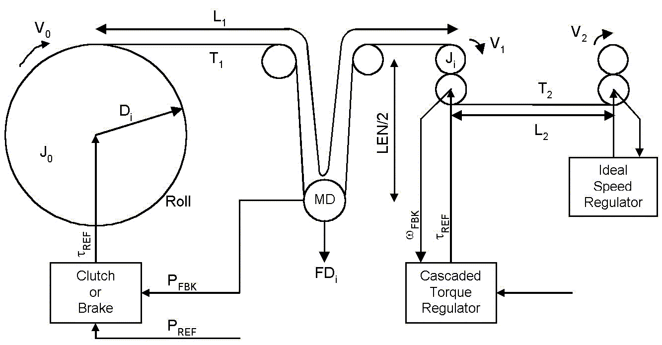
Figure 1. System Diagram
The ideal speed regulator provides the exit velocity for the second web span, a cascaded torque regulator (i.e. a torque regulator that is cascaded around a speed regulator) is included to dampen the dynamics between the stiff speed source and the winder/backstand dancer zone.
Nomenclature
sThe Laplace operator
J0The roll plus brake/clutch inertia [lb ft^2]
J1The motor + roll inertia of the cascaded torque regulated roll [lb ft^2]
ViThe i’th roll surface velocity [ft/min]
VDDancer velocity [ft/sec]
w iThe i'th roll rotational velocity feedback [rad/sec]
BVViscous friction [lb ft sec / rad]
BCCoulomb friction force [lb ft sec / rad]
BSStiction friction force [lb ft sec / rad]
RiThe i’th roll radius [ft]
RECEmpty core radius [ft]
RFRFull roll radius [ft]
GRiThe i’th roll gear ratio
LiThe i’th tension zone length [ft]
LENLength of material in dancer
LFixedLength of material in winder/backstand span minus material in dancer
TiThe i’th tension zone tension [lb]
t iThe i’th shaft torque [lb ft]
EiWeb modulus of elasticity [PSI]
EMODBase web Modulus of elasticity [PSI]
AiWeb cross sectional area [in^2]
WWeb width [ft]
d Material density [lb/ft^3]
THMaterial thickness [in]
NNumber of strands in the dancer
TSSample rate [sec]
First Principal Equations
The following equations describe the physical system.
Web Tension Equations
(1.1-4) describe the relationship between entry and exit web velocities and tension in a web span for the two web spans in the simulation of a winder.
 (1.1) (1.1)
 (1.2) (1.2)
For a backstand:
 (1.1a) (1.1a)
 (1.2a) (1.2a)
Where:
 (1.3) (1.3)
 (1.4) (1.4)
The proprietary non-linear equation f(Ti) describing the variation of web modulus of elasticity as a function of the web tension, or web strain to be more precise, closely mimics the non-linear behaviour of plastic non-deformable web material. The assumption is made that the strain in the material is limited such that deformation does not take place.
The non-linear power terms  are often ignored when modeling web processes. Ignoring these terms enables the integration algorithm to converge more quickly and results in faster simulation times. Given that this study is not prescribed to undertake a detailed study of web dynamics, and in order to facilitate a more rapid simulation, these terms have been dropped from the system simulation. are often ignored when modeling web processes. Ignoring these terms enables the integration algorithm to converge more quickly and results in faster simulation times. Given that this study is not prescribed to undertake a detailed study of web dynamics, and in order to facilitate a more rapid simulation, these terms have been dropped from the system simulation.
Torque Equations:
The equations describing the relationship between torque, rotational speed, and roll surface speeds are typically non-linear in nature. To assist in the description of these non-linear equations a linearized model is first described, then the modifications to the linearized model are presented.
 ; (1.5) ; (1.5)
The loss torque is a non-linear contribution that is a function of the magnitude and direction of the shaft speed. Equation (1.6) is a popular model that adequately represents the non-linear aspects of friction. It is from standard tribology texts on the subject.
 (1.6) (1.6)
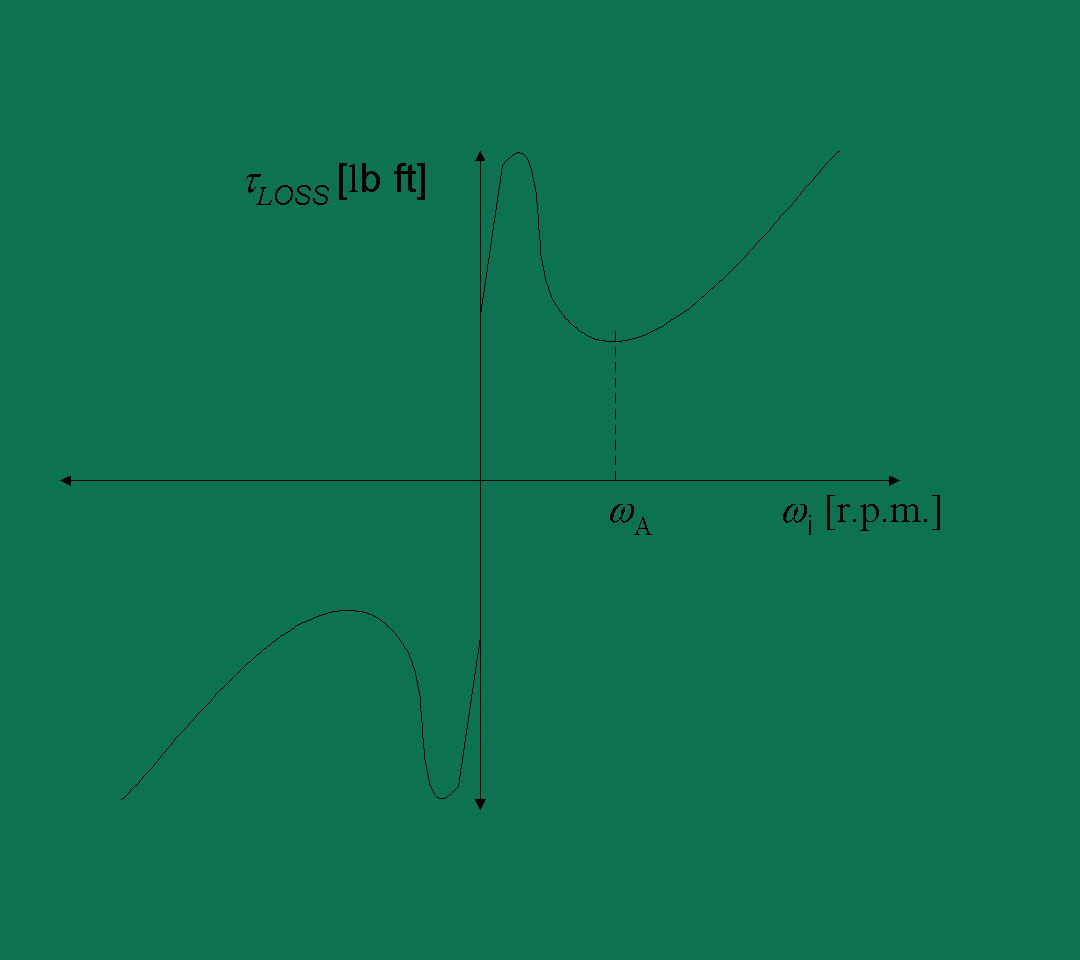
Figure 2. Graph of Typical Loss Torque shown in (1.6)
Only viscous friction was included in this simulation.
The Winder/Backstand torque equations have time varying inertia, and surface speed characteristics. The following equations describe this phenomena.
 ; (1.7) ; (1.7)
 ; (1.8) ; (1.8)
 ; (1.9) ; (1.9)
Dancer Force Balance Equations
Summing the forces at the dancer sub-system results in the following equations.
 (1.10) (1.10)
 (1.11) (1.11)
The proprietary fVD,T1 damping term is used to dampen high frequency instability in the integration algorithm that is used to solve the system of equations.
Simulation Controller structure
There are two regulators in the simulation;
- The dancer position regulation regulator
- The cascaded torque regulator
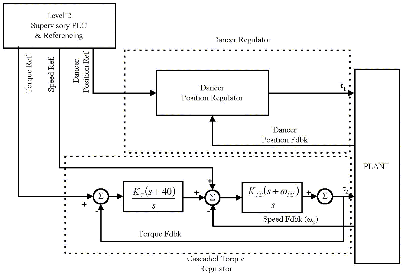
Figure 3. Controller Structure
Cascaded Torque Regulator
The cascaded torque regulator is tuned for a speed loop bandwidth of 5 [rad/sec] and a torque loop bandwidth of 5 [rad/sec].
Dancer Position Regulator
The adaptive non-linear dancer position regulator is proprietary and not described in this HTML version of the Report
SIMULATION STRUCTURE
Overview
The simulation is composed of two main sub-systems: The controller sub-system (yellow block) and the plant sub-system (blue block) as shown in Figure 9. Also included are references for line speed (magenta blocks) , wound-on tension, and creating dancer position steps (orange blocks). Scopes used for monitoring, and data storage blocks are represented by green blocks.
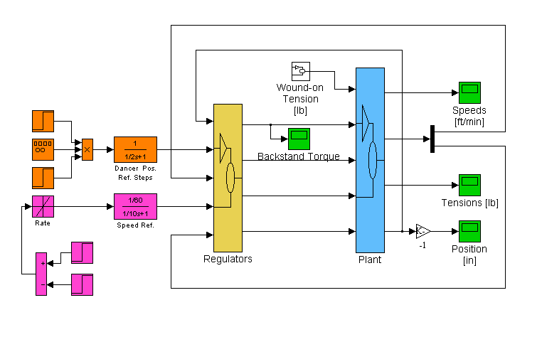
Figure 9. Simulation Main Block Diagram
Reference Generation
Two references are generated, a speed reference, and a dancer position reference. A winder wound-on tension reference can be used to investigate the effects of poor tension tapering in roll winding, for the investigation in this simulation it is set to zero. Following is a brief description of the speed and position references.
Speed Reference
The speed reference (magenta blocks) is generated with a pure ramp that is lagged with a 10 [rad/sec] lag. The ramp acceleration and deceleration rates are set in units of [f.p.m. / sec]. Using an S-Curve for the speed reference provided a slight improvement in the dancer position error at the beginning and end of the line acceleration, however it was not significant.
Position Reference
The default position reference was set at midpoint of the dancer range. A small position reference step train (orange blocks) was generated using a square wave generator. The magnitude of the steps was chosen such that the regulator torque reference did not saturate during the simulated run.
Plant sub-system
The plant sub-system is a block diagram of Eq’s (1.1) through (1.11) in Chapter 1 and is shown in Figure 10. The web equations are masked in the green blocks, and the torque equations are masked in the light blue blocks. The dancer force equations are masked in the magenta block. The web equations are coupled together with velocities, and the torque equations are coupled together with tensions as shown in Eq’s (1.1) through (1.11).
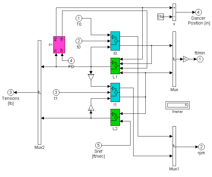
Figure 10. Plant Block Diagram
I0 Block Diagram
The I0 block diagram (Figure 11.) contains the torque equations describing the summation of torques in the backstand/winder system, and the change in diameter as a function of material thickness and rotational speed. (Eq's. 1.7-1.9).
The magenta blocks model the stiction phenomena that enables a backstand to produce a restraining torque. Briefly, the torque reference from the position controller can only produce a restraining torque when the roll is rotating. The magenta blocks that model this non-linear phenomena include magnitude limiting, rate limiting and square root gain blocks. Correctly setting these non-linear functions enables the simulation to closely mimic the non-linear friction behavior of a brake that is used to produce a restraining torque on a backstand. When simulating a clutch, the concept is the same except the torque is a motoring force and not a restraining force.
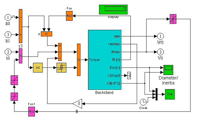
Figure 11. Backstand/Winder Block Diagram
The yellow blocks in Figure 11 model another friction phenomena known as static friction. Briefly, the differential load torque will not act on the system unless it exceeds a static friction value. This phenomena has a hysteresis characteristic that is modeled easily with a relay function. For more detailed explanations of these tribologic phenomena see [1], and [2].
Backstand Block Diagram
The backstand block is composed of the equations (1.5, 1.7 - 1.9) described in Chapter 1. It models the change in inertia as a function of roll diameter (magenta blocks). The roll diameter is modeled to vary as a function of rotational speed (yellow blocks). To simulate the effect of variations in roll diameter, the filtered rotational speed provides the once per rotation frequency for generating a sinusoidal disturbance to the roll diameter (cyan blocks). The torque divided by the Inertia [slugs] (orange blocks) is integrated to produce the roll rotational speed [rad/sec].
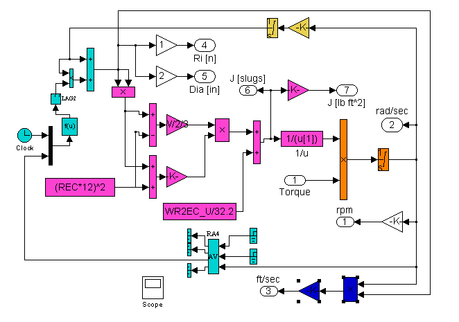
Figure 12. Backstand/Winder Block Diagram
L1 Block Diagram
L1 is a block diagram of Eq. (1.1). the blue blocks model the change in the T1 tension zone web length, as a function of dancer position Eq. (1.3). The magenta blocks represent the product of the non-linear E1 modulus of elasticity, and the cross sectional area. The dark blue block models the web material damping term Bw. The yellow blocks integrate the summed coupling velocities.
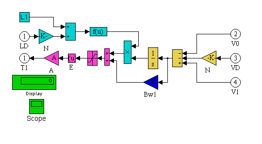
Figure 13. L1 Block Diagram
I1 Block Diagram
Figure 14. I1 block diagram models Eq. (1.5) for the cascaded torque regulated drive. No viscous damping was used in this section. The blue blocks integrate the summed torques acting on the roll inertia to produce a rotational speed [rad/sec]. The magenta blocks convert the rotational speed to a translational speed [ft/min].
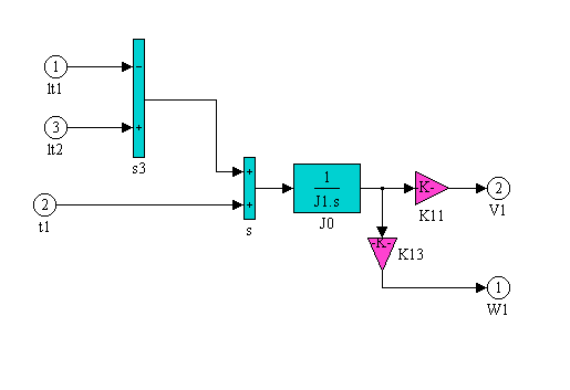
Figure 14. I1 Block Diagram
L2 Block Diagram
L2 is a block diagram of Eq (1.2). The magenta blocks represent the product of the non-linear E1 modulus of elasticity, and the cross sectional area. The dark blue block models the web material damping term Bw. The yellow blocks sum the coupling velocities and integrate them.
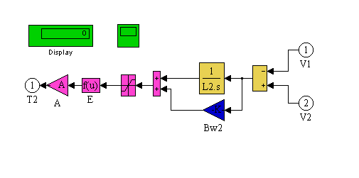
Figure 15. L2 Block Diagram
D1 Block Diagram
D1 block diagram represents a discrete model of the dancer Eq's. (1.10-11).
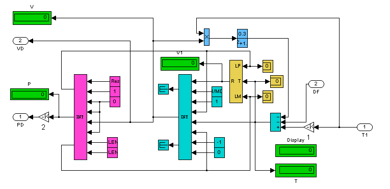
Figure 16. D1 Block Diagram
In the place of a continuous integrator model, ApICS LLC proprietary discrete integrators were used. This was done to enable the modeling of a movement bounded, velocity limited dancer. The dancer position in such a model will only operate between defined upper and lower limits. This was accomplished using the limit logic and clamping features of the integrators. Following is a description of the model:
The cyan blocks integrate the summation of forces acting on the dancer and calculate the dancer velocity. The cyan integrator gain is equal to 1/MD or the inverse of the dancer mass [slugs]. The output of this integrator, and by implication the dancer speed, is limited to +/- 1 [ft/sec] which is reasonable for these applications. The unity gain magenta integrator block integrates the velocity to produce the dancer position. The dancer position is limited between 0 and -LEN [ft]. The initial condition of the integrator is set at -LEN (or hard down). The yellow block contains the logic used to reset the velocity integrator to zero when a position limit is reached, and release it when the dancer forces sum in such a way that the dancer moves from the given limit. The blue block contains a proprietary damping function that dampens high frequency numerical instability in the integration algorithm.
Regulators Sub-System
There are two controllers (Figure 17.) in the system. A cascaded torque controller for the drive that is used to isolate the ideal speed reference from the winder/backstand tension zone, and the non-linear adaptive dancer position regulator. Both of the controllers are modeled in the simulation with blocks that are implemented as discrete s-functions. The s-functions are written with difference equations and internal logic that exactly replicate the behavior of sampled digital control systems, including quantization errors.
The blue block represents the cascaded torque regulator, the yellow block represents the dancer position regulator. The orange block contains a model of the brake/clutch lag and transport delay. The magenta blocks provide a dancer load force reference. The load force reference is scaled such that it reaches full dancer force from zero in 1 [sec] regardless of the force set-point.
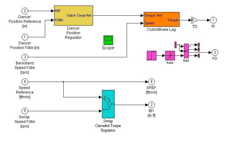
Figure 17. Regulators Block Diagram
Cascaded Torque Regulator Block Diagram
(Figure 18) normalization (orange blocks) of the speed and torque references and feedbacks is used to so that the regulator can be tuned in a per-normal manner. The speed (cyan block) and torque (magenta blocks) regulators are tuned for a bandwidth of 5 [rad/sec]. The Torque reference is set to zero, therefore there is no tension difference between T1 and T2 when running at a constant line speed. Because there is no inertia compensation used in the torque regulator there is a small tension difference between T1 and T2 during acceleration and deceleration.
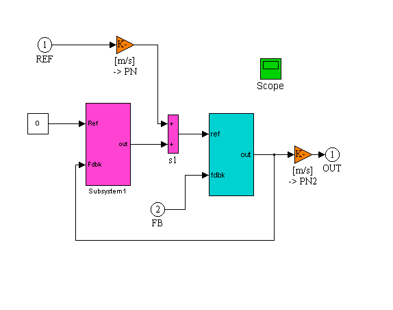
Figure 18. Cascaded Torque Regulator (CTR) Block Diagram
CTR Speed Regulator Block Diagram
The CTR speed loop block diagram is shown in Figure 19.
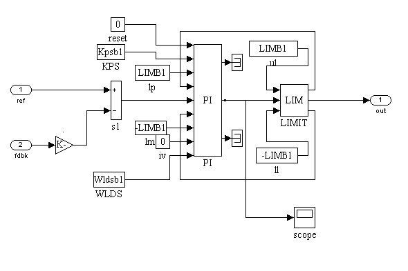
Figure 19. CTR Speed Regulator Block Diagram
CTR Torque Regulator Block Diagram
The CTR torque loop block diagram is shown in Figure 20.
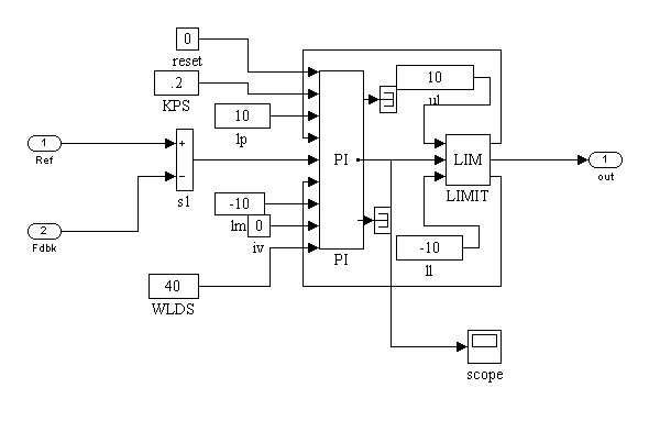
Figure 20. CTR Torque Regulator Block Diagram
Dancer Position Regulator Block Diagram
The dancer position regulator block diagram is protected by an IP agreement and is not shown in this HTML version of the report
RESULTS
Overview
Three sets of simulation results are presented.
- The first set presents the results from simulations of unwinding with a backstand brake. These results show the efficacy of the gain and frequency 2nd order controller adaptation algorithms during a full wind-down of a roll from 60 [in] to approx. 3 [in] for a variety of web thicknesses and modulus.
- The second set presents results from simulations of winding with a clutch drive. These results show the efficacy of the gain and frequency 2nd order controller adaptation algorithms during a full windup of a roll from 3 [in] to approx. 60 [in].
- The third set of simulations present results that demonstrate the efficacy of the gain adaptation algorithm at a set of various starting winding diameters. This set of simulation plots are of 40 [sec] duration and show the behavior of the controller at machine start-up and during line acceleration.
For most of the results, the following plots are presented for each result set.
- Dancer position [in],
- Web Tensions [lb]
- Backstand/Winder torque [lb ft]
- Line speed [ft/min]
- Roll Diameter [in], and Inertia [lb ft2]
Other than those indicated by the plots, the parameters found in Appendix A were used during the simulation:
Unwinding, .005 [in^2}, 0.01 [lb/in^3} W=24 [in]

Figure 25. Dancer Position, U, .005 [in^2}, 0.01 [lb/in^3} W=24 [in]
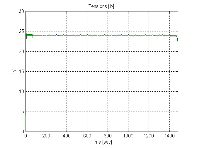
Figure 26. Web Tensions, U, .005 [in^2}, 0.01 [lb/in^3} W=24 [in]
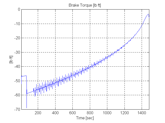
Figure 27. Backstand Torque, U, .005 [in^2}, 0.01 [lb/in^3} W=24 [in]
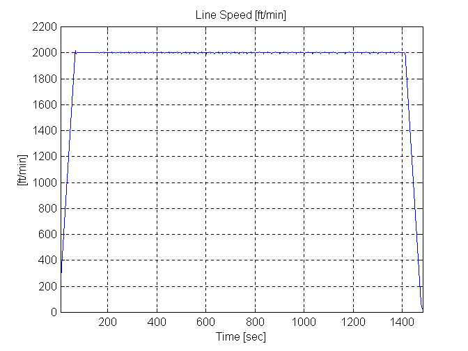
Figure 28. Line Speed, U, .005 [in^2}, 0.01 [lb/in^3} W=24 [in]
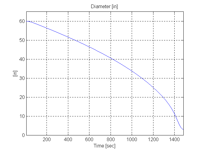
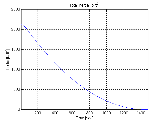
Figure 29. Diameter & Inertia, U, .005 [in^2}, 0.01 [lb/in^3} W=24 [in]
Unwinding, .01 [in^2}, 0.01 [lb/in^3} W=24 [in]
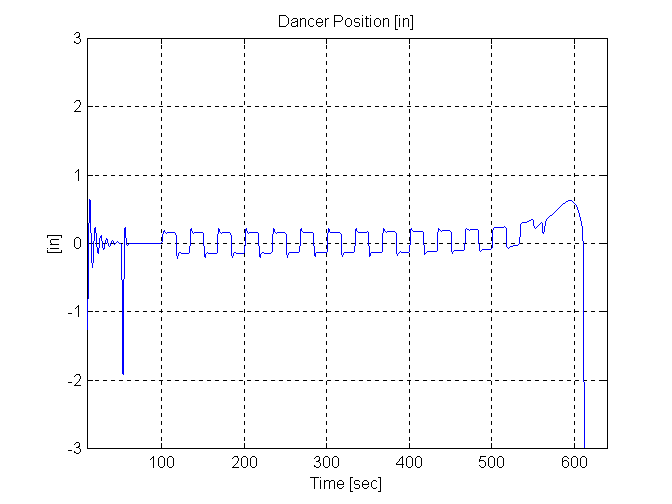
Figure 30. Dancer Position, U, .01 [in^2}, 0.01 [lb/in^3} W=24 [in]
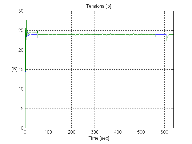
Figure 31. Web Tensions, U, .01 [in^2}, 0.01 [lb/in^3} W=24 [in]
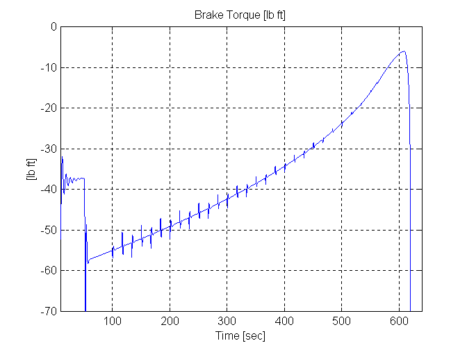
Figure 32. Backstand Torque, U, .01 [in^2}, 0.01 [lb/in^3} W=24 [in]
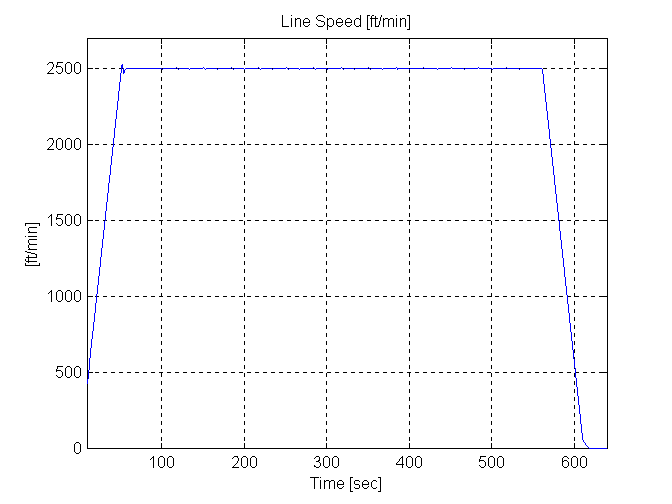
Figure 33. Line Speed, U, .01 [in^2}, 0.01 [lb/in^3} W=24 [in]

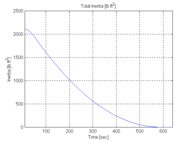
Figure 34. Diameter & Inertia, U, .01 [in^2}, 0.01 [lb/in^3} W=24 [in]
Unwinding, .01 [in^2}, 0.005 [lb/in^3} W=24 [in]
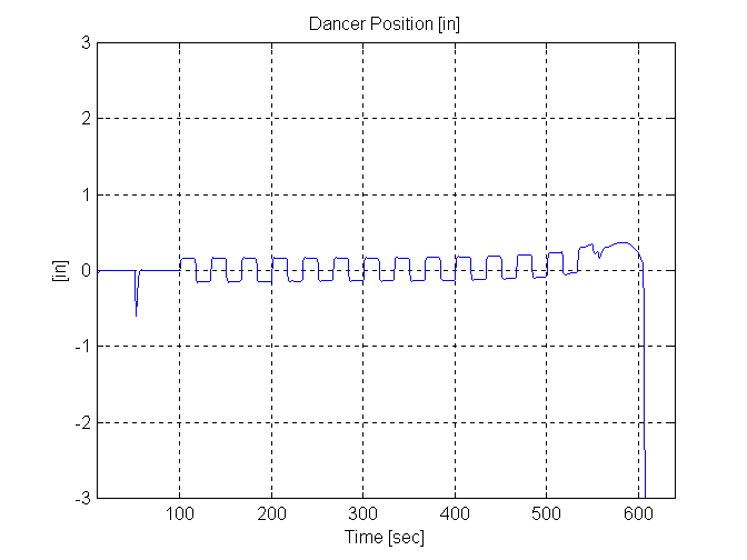
Figure 35. Dancer Position, U, .01 [in^2}, 0.005 [lb/in^3} W=24 [in]
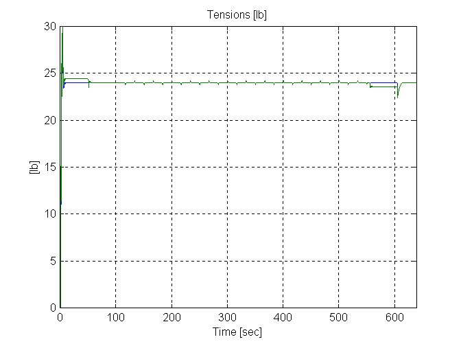
Figure 36. Web Tensions, U, .01 [in^2}, 0.005 [lb/in^3} W=24 [in]
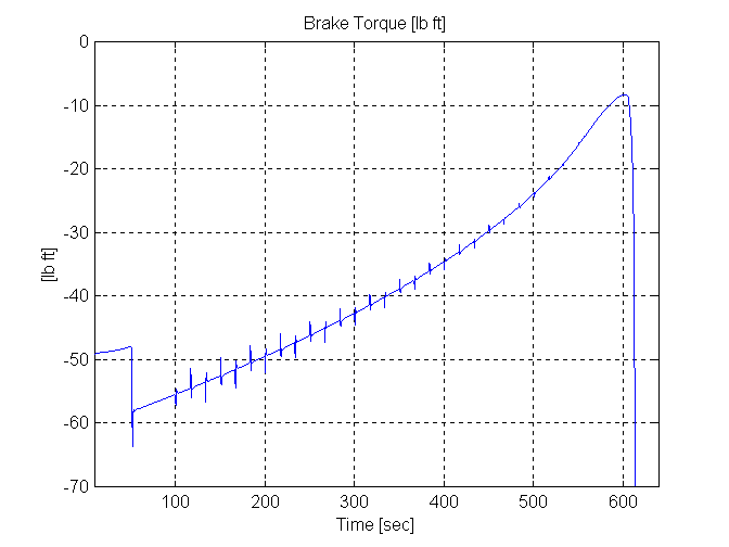
Figure 37. Backstand Torque, U, .01 [in^2}, 0.005 [lb/in^3} W=24 [in]
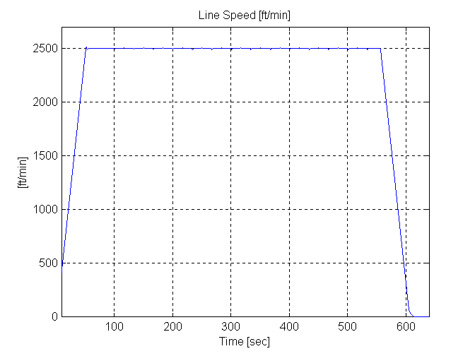
Figure 38. Line Speed, U, .01 [in^2}, 0.005 [lb/in^3} W=24 [in]
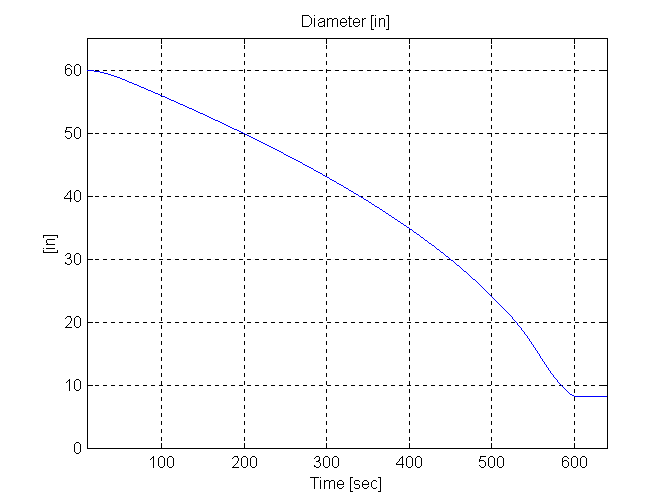
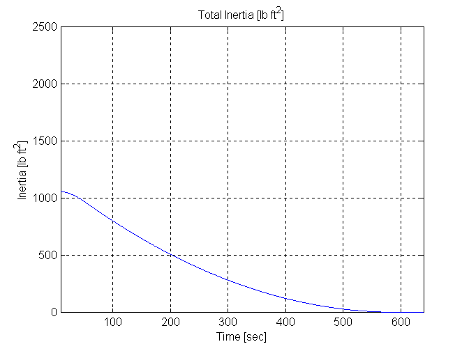
Figure 39. Diameter & Inertia, U, .01 [in^2}, 0.005 [lb/in^3} W=24 [in]
Unwinding, .01 [in^2}, 0.015 [lb/in^3} W=12 [in]
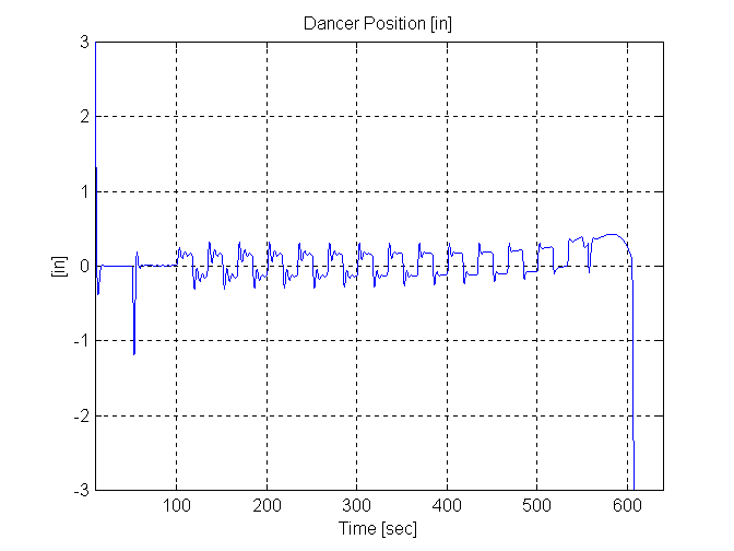
Figure 40. Dancer Position, U, .01 [in^2}, 0.015 [lb/in^3} W=12 [in]
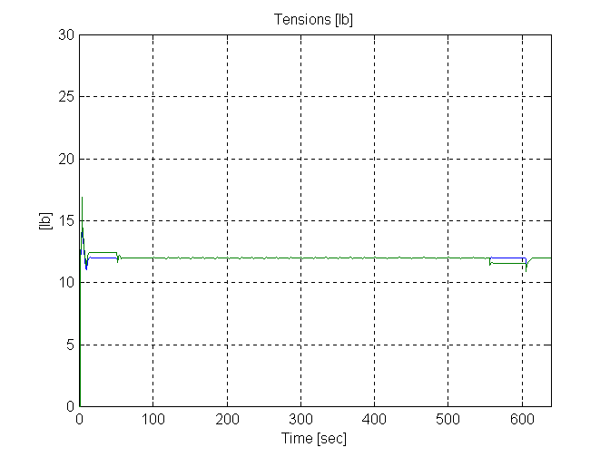
Figure 41. Web Tensions, U, .01 [in^2}, 0.015 [lb/in^3} W=12 [in]
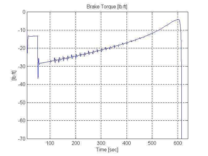
Figure 42. Backstand Torque, U, .01 [in^2}, 0.015 [lb/in^3} W=12 [in]
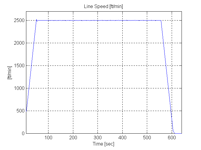
Figure 43. Line Speed, U, .01 [in^2}, 0.015 [lb/in^3} W=12 [in]


Figure 44. Diameter & Inertia, U, .01 [in^2}, 0.015 [lb/in^3} W=12 [in]
Unwinding, .01 [in^2}, 0.015 [lb/in^3} W=6 [in]
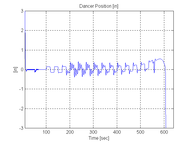
Figure 45. Dancer Position, U, .01 [in^2}, 0.015 [lb/in^3} W=6 [in]
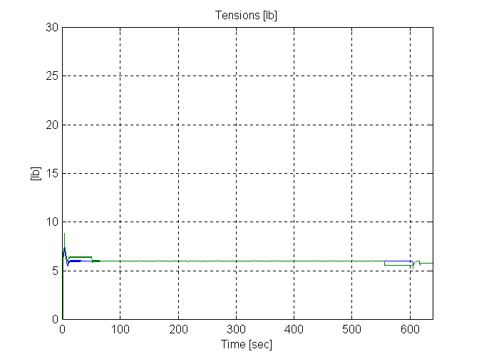
Figure 46. Web Tensions, U, .01 [in^2}, 0.015 [lb/in^3} W=6 [in]
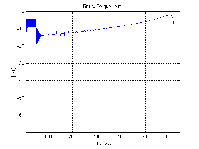
Figure 47. Backstand Torque, U, .01 [in^2}, 0.015 [lb/in^3} W=6 [in]
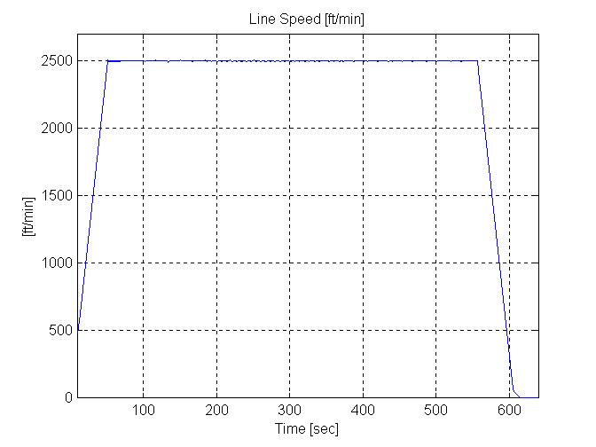
Figure 48. Line Speed, U, .01 [in^2}, 0.015 [lb/in^3} W=6 [in]

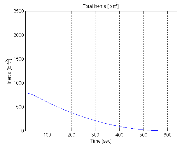
Figure 49. Diameter & Inertia, U, .01 [in^2}, 0.015 [lb/in^3} W=6 [in]
Unwinding, .01 [in^2}, 0.015 [lb/in^3} W=36 [in]
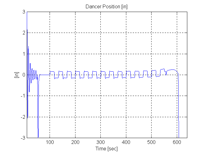
Figure 50. Dancer Position, U, .01 [in^2}, 0.015 [lb/in^3} W=36 [in]
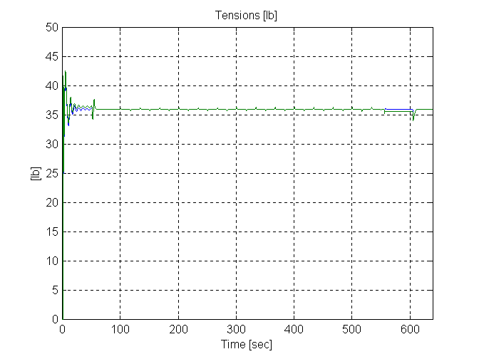
Figure 51. Web Tensions, U, .01 [in^2}, 0.015 [lb/in^3} W=36 [in]
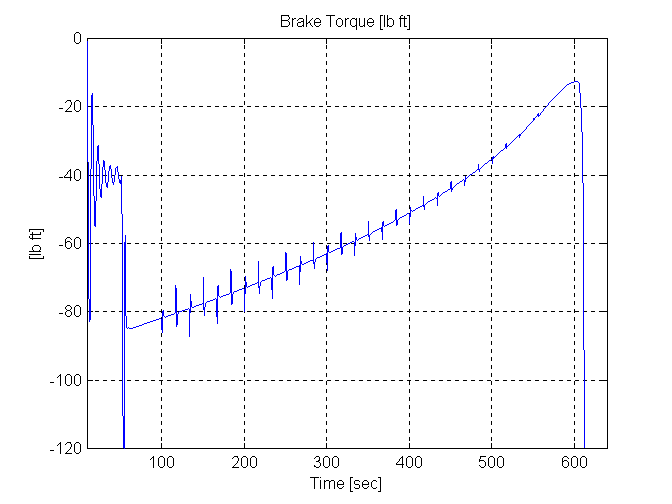
Figure 52. Backstand Torque, U, .01 [in^2}, 0.015 [lb/in^3} W=36 [in]
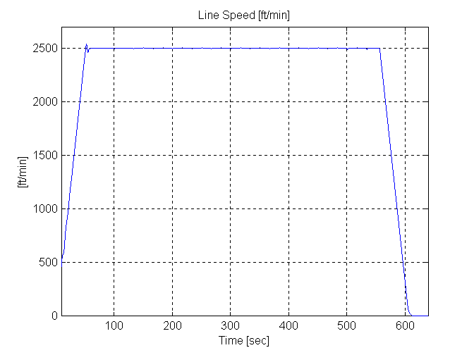
Figure 53. Line Speed, U, .01 [in^2}, 0.015 [lb/in^3} W=36 [in]


Figure 54. Diameter & Inertia, U, .01 [in^2}, 0.015 [lb/in^3} W=36 [in]
Winding, .01 [in^2}, 0.01 [lb/in^3} W=36 [in]
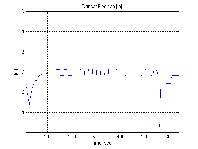
Figure 55. Dancer Position, U, .01 [in^2}, 0.01 [lb/in^3} W=36 [in]
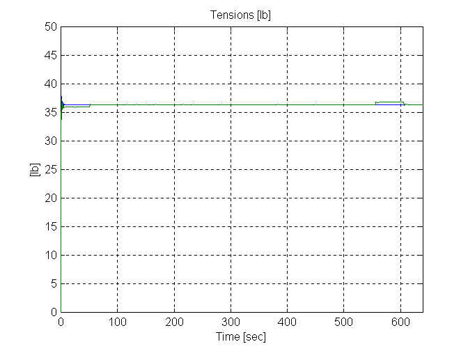
Figure 56. Web Tensions, U, .01 [in^2}, 0.01 [lb/in^3} W=36 [in]
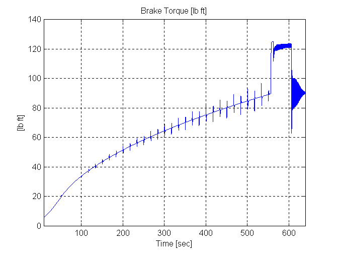
Figure 57. Winder Torque, U, .01 [in^2}, 0.01 [lb/in^3} W=36 [in]

Figure 58. Line Speed, U, .01 [in^2}, 0.01 [lb/in^3} W=36 [in]
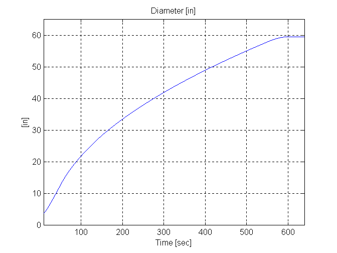

Figure 59. Diameter & Inertia, U, .01 [in^2}, 0.01 [lb/in^3} W=36 [in]
Winding, .01 [in^2}, 0.01 [lb/in^3} W=24 [in]
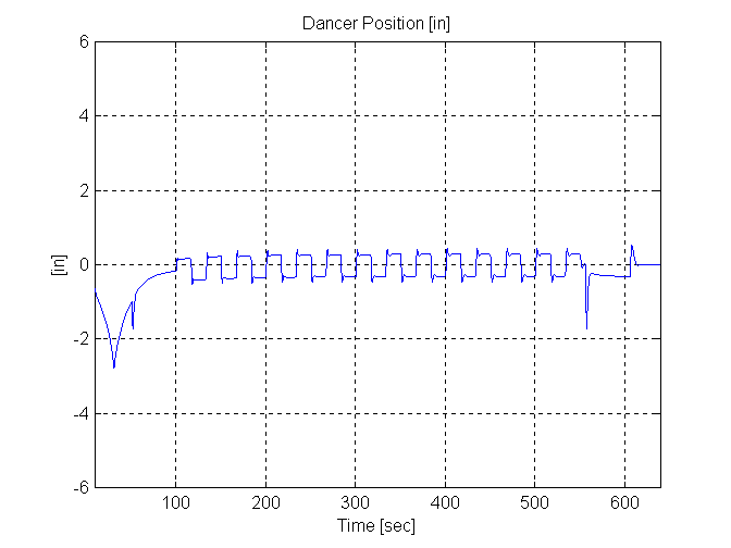
Figure 60. Dancer Position, U, .01 [in^2}, 0.01 [lb/in^3} W=24 [in]
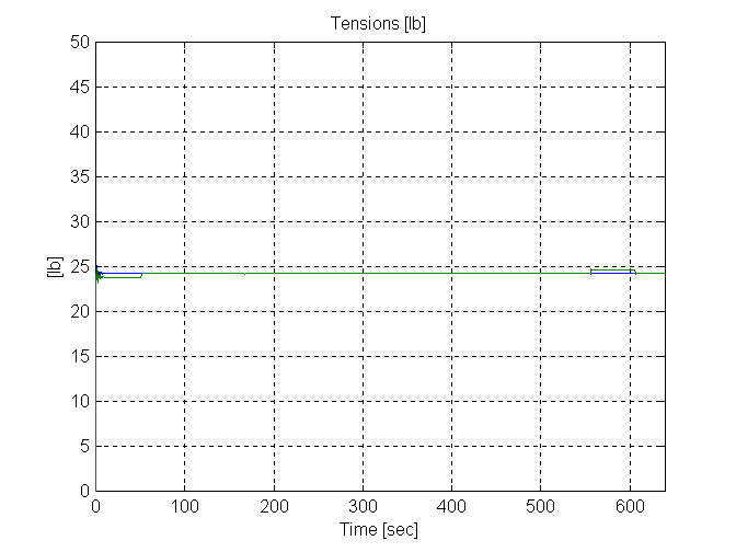
Figure 61. Web Tensions, U, .01 [in^2}, 0.01 [lb/in^3} W=24 [in]
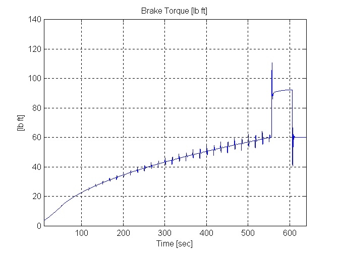
Figure 62. Winder Torque, U, .01 [in^2}, 0.01 [lb/in^3} W=24 [in]
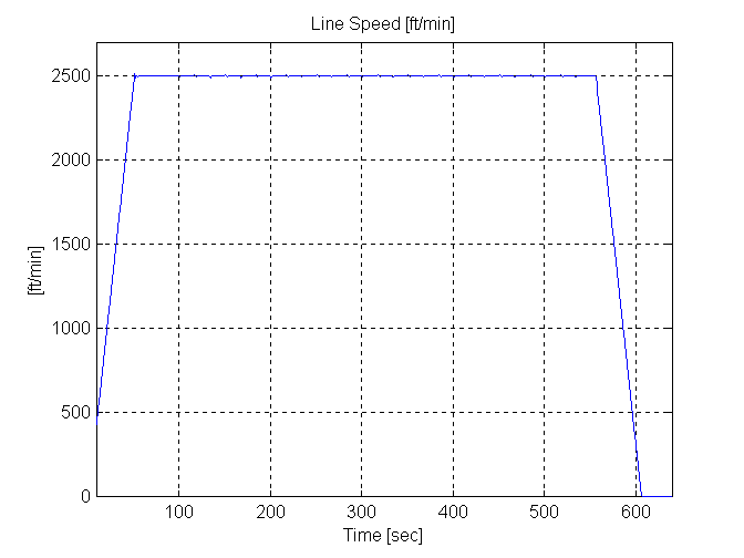
Figure 63. Line Speed, U, .01 [in^2}, 0.01 [lb/in^3} W=24 [in]

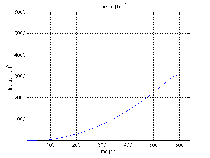
Figure 64. Diameter & Inertia, U, .01 [in^2}, 0.01 [lb/in^3} W=24 [in]
Winding, .01 [in^2}, 0.015 [lb/in^3} W=12 [in]
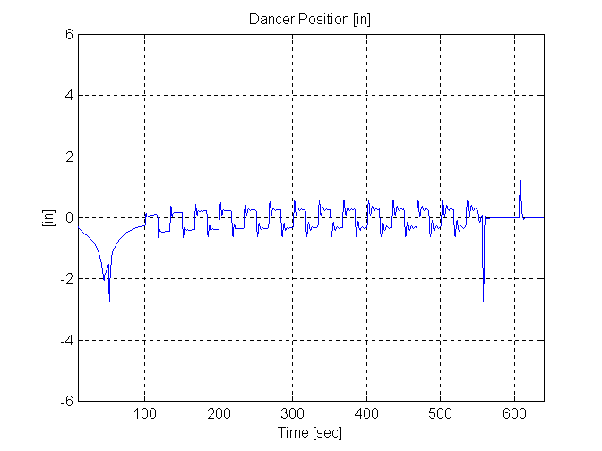
Figure 70. Dancer Position, U, .01 [in^2}, 0.015 [lb/in^3} W=12 [in]
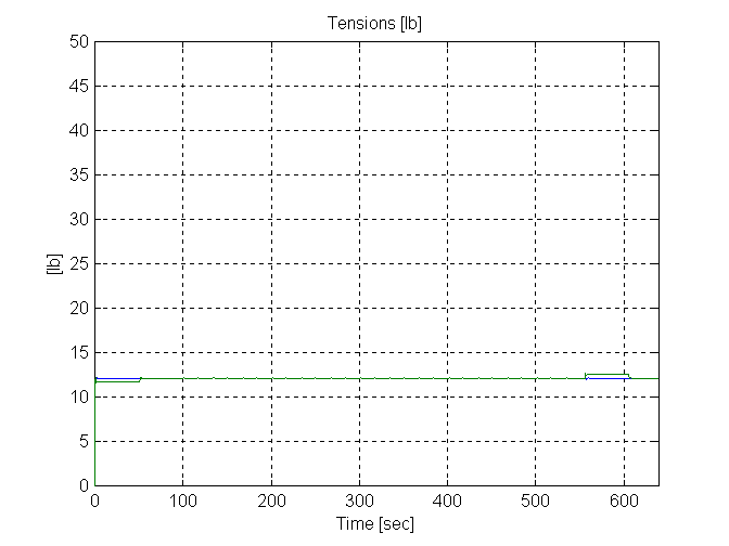
Figure 71. Web Tensions, U, .01 [in^2}, 0.015 [lb/in^3} W=12 [in]
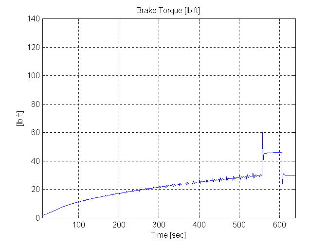
Figure 72. Winder Torque, U, .01 [in^2}, 0.015 [lb/in^3} W=12 [in]

Figure 73. Line Speed, U, .01 [in^2}, 0.015 [lb/in^3} W=12 [in]


Figure 74. Diameter & Inertia, U, .01 [in^2}, 0.015 [lb/in^3} W=12 [in]
Winding, .01 [in^2}, 0.015 [lb/in^3} W=6 [in]

Figure 75. Dancer Position, U, .01 [in^2}, 0.015 [lb/in^3} W=6 [in]
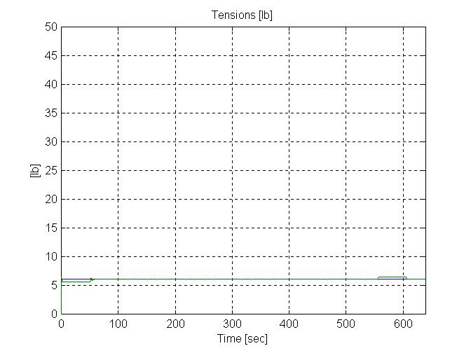
Figure 76. Web Tensions, U, .01 [in^2}, 0.015 [lb/in^3} W=6 [in]
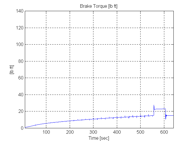
Figure 77. Winder Torque, U, .01 [in^2}, 0.015 [lb/in^3} W=6 [in]
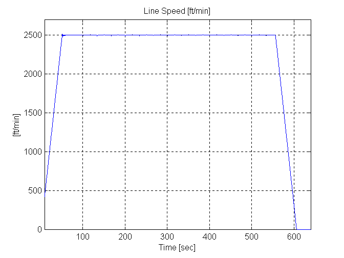
Figure 78. Line Speed, U, .01 [in^2}, 0.015 [lb/in^3} W=6 [in]

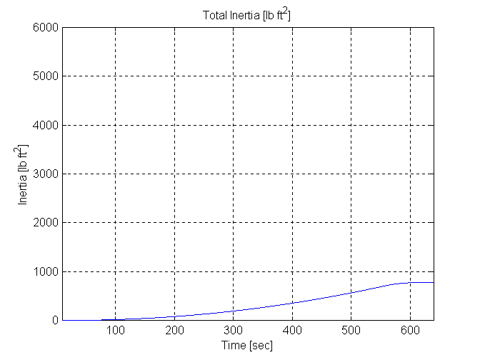
Figure 79. Diameter & Inertia, U, .01 [in^2}, 0.015 [lb/in^3} W=6 [in]
Unwinding, .01 [in^2}, 0.015 [lb/in^3} D=60 [in], 40 [sec]
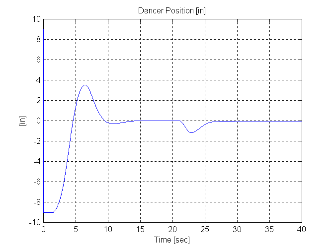
Figure 80. Dancer Position, U, .01 [in^2}, 0.015 [lb/in^3} D=60 [in]
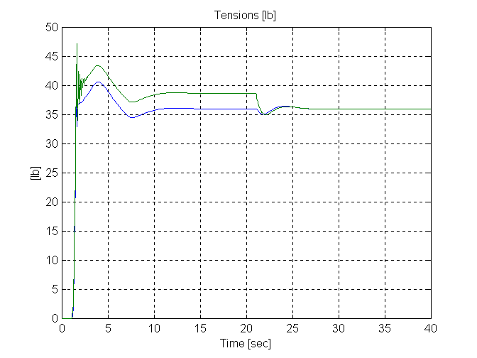
Figure 81. Web Tensions, U, .01 [in^2}, 0.015 [lb/in^3} D=60 [in]
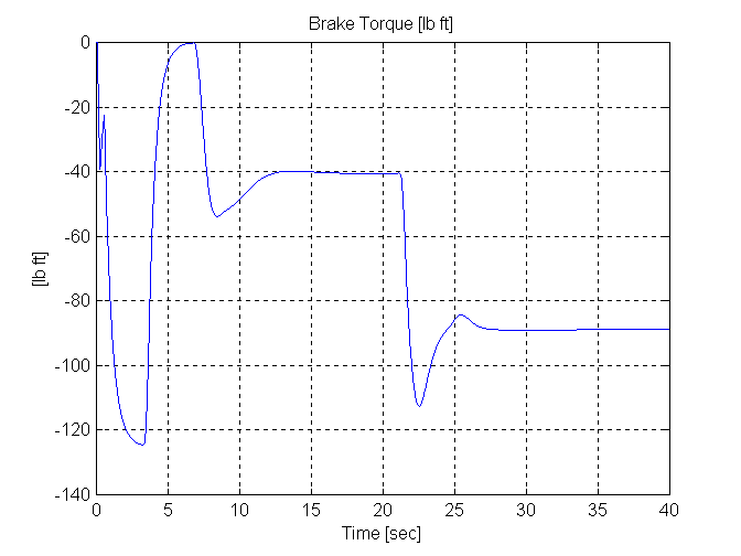
Figure 82. Backstand Torque, U, .01 [in^2}, 0.015 [lb/in^3} D=60 [in]
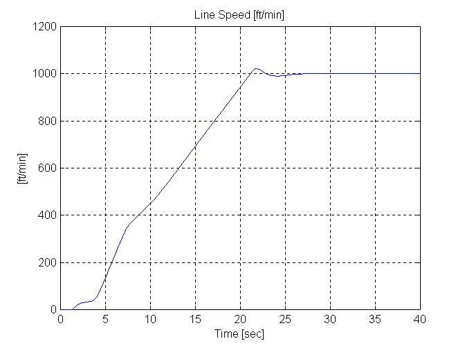
Figure 83. Line Speed, U, .01 [in^2}, 0.015 [lb/in^3} D=60 [in]
Unwinding, .01 [in^2}, 0.01 [lb/in^3} D=30 [in], 40 [sec]
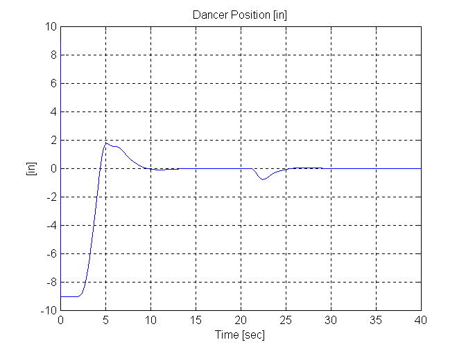
Figure 84. Dancer Position, U, .01 [in^2}, 0.01 [lb/in^3} D=30 [in]
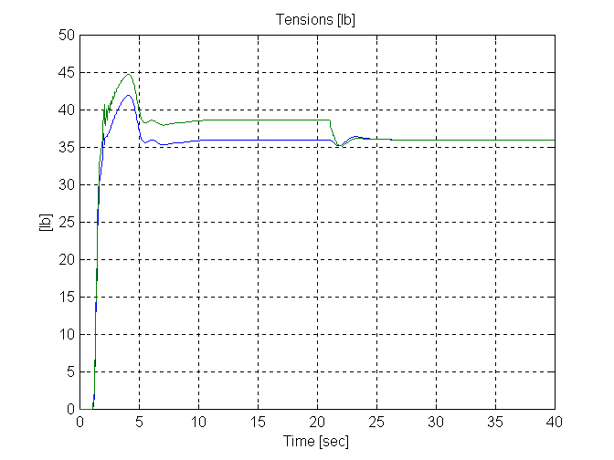
Figure 85. Web Tensions, U, .01 [in^2}, 0.01 [lb/in^3} D=30 [in]
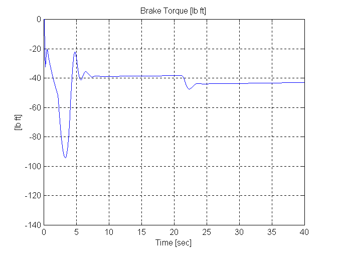
Figure 86. Backstand Torque, U, .01 [in^2}, 0.01 [lb/in^3} D=30 [in]
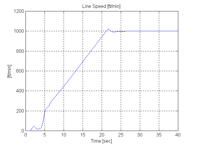
Figure 87. Line Speed, U, .01 [in^2}, 0.01 [lb/in^3} D=30 [in]
Unwinding, .01 [in^2}, 0.015 [lb/in^3} D=12 [in], 40 [sec]
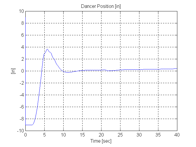
Figure 88. Dancer Position, U, .01 [in^2}, 0.015 [lb/in^3} D=12 [in]
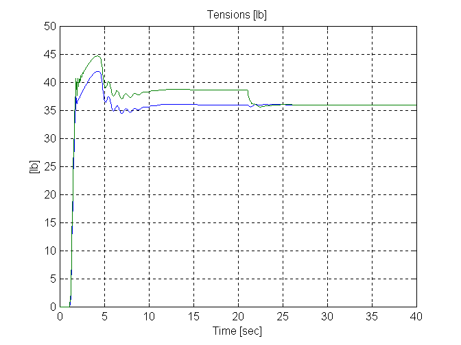
Figure 89. Web Tensions, U, .01 [in^2}, 0.015 [lb/in^3} D=12 [in]
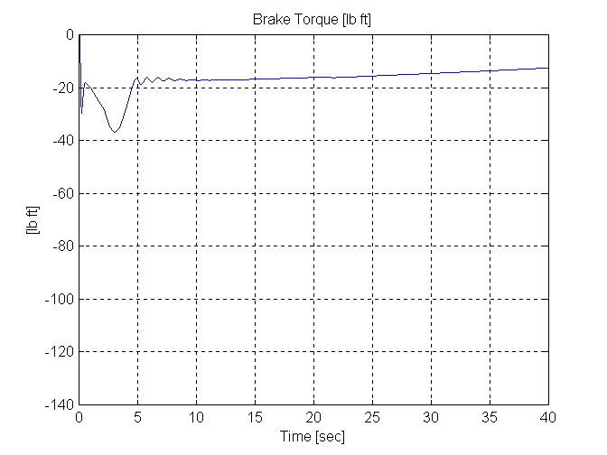
Figure 90. Backstand Torque, U, .01 [in^2}, 0.015 [lb/in^3} D=12 [in]

Figure 91. Line Speed, U, .01 [in^2}, 0.015 [lb/in^3} D=12 [in]
Unwinding, .01 [in^2}, 0.015 [lb/in^3} D=6 [in]
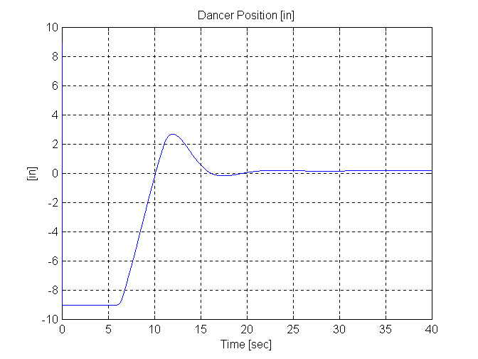
Figure 92. Dancer Position, U, .01 [in^2}, 0.015 [lb/in^3} D=6 [in]
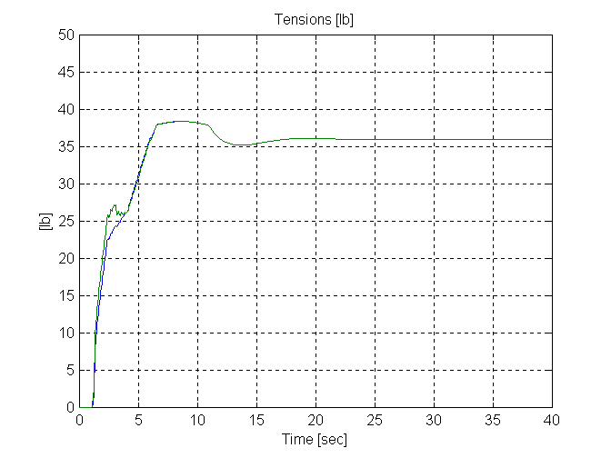
Figure 93. Web Tensions, U, .01 [in^2}, 0.015 [lb/in^3} D=6 [in]
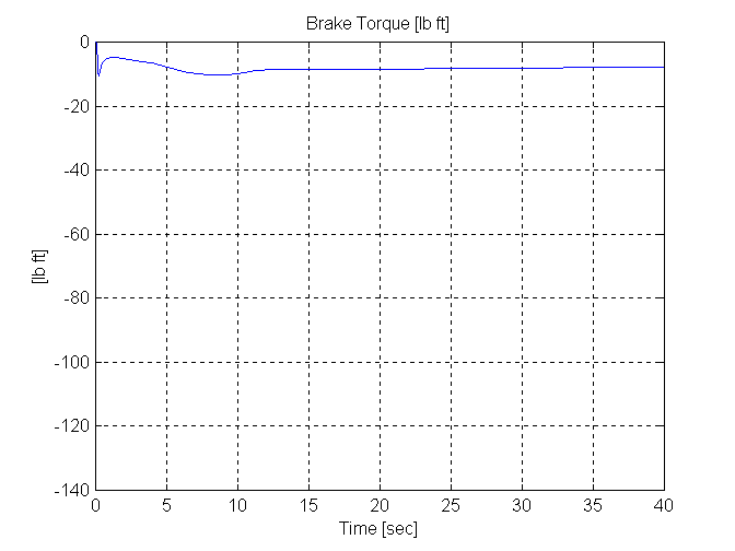
Figure 94. Backstand Torque, U, .01 [in^2}, 0.015 [lb/in^3} D=6 [in]
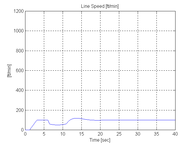
Figure 95. Line Speed, U, .01 [in^2}, 0.015 [lb/in^3} D=6 [in]
CHAPTER 4
SEQUENCING ISSUES & START-UP PROCEDURES
This section of the report is proprietary and not included in the HTML version of the report
BIBLIOGRAPHY
[1]Hess, D.P., Soom, A. "Friction at a Lubricated Line Contact Operating at Oscillating Sliding Velocities" Journal of Tribology Transactions of the ASME Vol 112, pp 147-152, 1992.
[2] Majd, V.J.. Simaan M. A., "A Continuous Friction Model For Servo Systems With Stiction", Proceedings of the 4th I.E.E.E. Conference on Control Applications, Albany NY. 1996
|