Applied Industrial Control Solutions LLC
ApICS LLC.
A Modular, Autonomous Naval Heavy Ordnance Handling System
and
Positioning / Motion Control Regulator Design
B. T. Boulter
© ApICS ® LLC 2000
ABSTRACT
This study describes the first principal equations used to prescribe a simulation of a "Modular, Autonomous Heavy Ordnance Handling Systems". The study was commisioned by Orbital Research INC (OH). Sets of results that reflect the expected system performance are provided. Included is a brief description of the simulation sub-systems. The simulation description is meant to provide the user with the information required to perform "what-if" scenarios using the simulation.
INTRODUCTION
Scope
The scope of this document is limited to describing the first principal equations describing the system, and to providing an overview of the simulation and the control structure sub-systems.
Results
Sets of results that provide insight into the expected behavior of the system with varying system plant and controller parameters are included.
For each presented result, a set of plots including, Handler Position error [cm], Speeds v0, v1, v2, [m/s], K1, K2, Damper Forces [N] F1, F2, Motor Forces [N] (see Figure 1.) are reported. The investigations include: the effect of damper stiffness, the effect of tuning, the effect of a height disturbance, and the effect of wave motion, on the dynamics of the positioning system tracking response.
The study concludes with some pertinent observations, and conclusions/recommendations.
PLANT FIRST PRINCIPAL EQUATIONS
OVERVIEW
Figure 1. describes the mass spring approximation of the system under study. Equations (1.1) through (1.8) describe the system shown in figure 1, with the inclusion of non-linear relationships between state variables that are not obvious from the figure.
Figure 1. Mass-Spring Diagram
First Principal Equations
The following equations describe the physical system. (1.1) describes the linear relationship between momentum, speed and position of the handler mass. A force DF that results from the effect of wave motion on the handler momentum in the translational plane of carriage motion is included:
 (1.1) (1.1)
 (1.1a) (1.1a)
It can be shown that the force DF that results from the effect of wave action is modeled as shown in (1.1a) with a frequency of w2 [r/s] and a max. amplitude of Bv [N] with an initial phase of f2 [r].
The handler offset angle (i.e. the misalignment in the translational plane of motion) between the upper and lower rails) is given as:
 (1.2) (1.2)
The change in height between the upper and lower rails is described as:
 (1.3) (1.3)
 (1.4) (1.4)
Where: w1 = desired disturbance frequency [r/s] with intial phase of f and amplitude of A [m]
After making several assumptions, K1 and K2 are assumed to be non-linearly dependant on the offset angle q of the handler, and the screw down force of the damper/springs. In addition, the screw down force of the damper springs is understood to vary with the height differential Dh between the top and bottom drive railings. This height variation (1.3,4) is a sinusoidal disturbance that varies in amplitude and frequency as the vessel structure is excited by the forces introduced by the action of ocean waves. Therefore:
 (1.5) (1.5)
As shown in (1.5) above, the change is the spring constant as a function of handler angle q, and height differential Dh are assumed to be simple signum power functions.
The angle of the ship, and by consequence the handler, will impact frictional forces and loading on the carriage rails. The following equations describe the impact of the vessel angle  , handler offset angle q, and height differential Dh, on a fixed stiction (static friction, similar to the change in K shown in Figure 4.) force acting on the rails: , handler offset angle q, and height differential Dh, on a fixed stiction (static friction, similar to the change in K shown in Figure 4.) force acting on the rails:
 (1.6) (1.6)
The static friction force offset due to wave motion is modeled with a frequency of w2 [r/s] and a max. amplitude of OB [N] with an initial phase of f2 [r]. Eqn’s (1.7,8) describe the linear relationship between momentum, speed and position of the linear motor carriage masses, the driving forces, and the approximated impairing stiction forces:
 (1.7,8) (1.7,8)
A proprietary damping function  is deployed to suppress high frequency resonance phenomena. This function does not effect the response of the system in the frequency range of interest. It is used to provide the integration algorithm with numerical stability in the high frequency spectra region of the simulation. is deployed to suppress high frequency resonance phenomena. This function does not effect the response of the system in the frequency range of interest. It is used to provide the integration algorithm with numerical stability in the high frequency spectra region of the simulation.
Controller structure
The controller structure in this application is limited by the choice of the linear motor drive that is being used. The drive that has been chosen for this application (TBD) has a fixed controller structure that is not programmable. A custom control architecture could be implemented in a programmable drive, such as a Rockwell Automation Automax DPS drive, or a Drivelogix programmable drive, however these drives are significantly more costly than their simpler fixed structure counterparts, and will not be used in this application.
Although a programmable GE Fanuc PLC is being used for supervisory control, it is not feasible to close loops using A/D’s and D/A’s with this PLC. The combination of asynchronous communications and insufficient scan times will result in aliasing and Nyquist frequency limitations that will significantly reduce the headroom of the loop bandwidths. Given that the drive that is to be used in the proof of feasibility will, for the time being, only allow for a fixed architecture, the simulation has been structured to reflect that architecture.
Figure 2 outlines the basic controller structure. Each amplifier consists of a cascaded position and speed loop. A feed-forward speed reference and inertia/momentum compensation signal are derived from the position reference. Because derivatives are used to obtain these feed-forward signals, it is usually desirable to deploy a synchronized digital position reference that is clean. In most drives this is achieved by supplying a reference level, and a start command. The drive then internally generates its own references. If however, an external analog position reference is used, the feed-forward signals will usually be corrupted by noise and unusable, resulting in significantly degraded loop command reference response. For this reason it is not recommended to use an analog position reference.
The position and speed loop PI’s are represented in their frequency domain format. The PI integral gain can be obtained from the lead frequency as follows: wld = Ki / Kp -> Ki = wld * Kp.
Using normalized tuning methods, the tuning equations in the following sections are used to tune the regulators:
Figure 2. Controller Structure
Tuning Equations Overview
Some definitions used in the tuning equations follow. If a normalized structure is used in the regulators, the tuning of the speed and position regulators is greatly simplified. Another benefit of this tuning approach is that the bandwidths of the various regulators can be determined without the need for step tests. Briefly, a regulator is normalized if the reference has a value of 1 at rated speed (SMAX) or position (PMAX), and similarly, the feedback is scaled such that it has a value of 1 at the same rated speed or position. The torque/force reference should then be scaled such that it has a value of 1 at rated force or torque (FMAX). If this method is used to normalize the regulators, the following tuning equations apply:
Per-Normal Inertia/Mass
Figure 3. shows that Per-normal reflected inertia/mass [sec] is the time in seconds that it takes to accelerate the motor and load inertia/mass from zero speed to rated motor speed (Sb) with motor rated torque/force (tRated) and the given reflected inertia/mass.
Figure 3. Per-Normal Inertia [sec]
Speed Loop Tuning
SMAX= 5;% Max Rail Speed [m/s]
FMAX= 660;% Max Rail Force [N]
J_U= (m0+m1)/(FMAX)*SMAX;% J_Bar of upper track [s]
J_L= (m0+m2)/(FMAX)*SMAX;% J_Bar of lower track [s]
WCOUS= 40;% Desired speed loop bandwidth [r/s]
KPUS= WCOUS*J_U;% Speed loop prop. gain []
WLDUS= WCOUS/5;% Speed loop lead freq. [r/s]
Position Loop Tuning
Similar to the concept of a per-normal inertia/mass in the tuning of a speed loop, the position loop can be tuned with a per-normal time constant. Briefly, P_Bar is the time it takes in seconds to travel from zero to rated position at rated speed. For example if the feedback is scaled such that 1 in the feedback and reference of the normalized position regulator is equivalent to 3 [m], and the max speed is 5 [m/s], P_Bar = 5/3 = 1 2/3 [sec].
PMAX= 3;% Max Rail Position [m]
P_U= PMAX/SMAX;% P_Bar [sec]
WCOUP= 15;% Desired position loop bandwidth [r/s]
KPUP= WCOUP*P_U;% Position PI prop. gain []
WLDUP= WCOUP/3;% Position PI lead freq. [r/s]
Determining non-linear equation coefficients
The coefficients used in the non-linear equations in the simulation can be obtained using empirical data obtained from the machine or, if this is not feasible, good engineering judgement. Given that the machine is not built yet, we shall have to resort to good engineering judgement.
B1 and B2
B1 and B2 were sized such that, with all loops disabled, the mass-spring natural frequency dampens within 1 [sec]. After stepping the Force input and adjusting for the above damping time, B1 = B2 = 1000 [N*s/m]
K1 and K2
The simulation is robust for a range of base spring constant stiffness of 1 – 1000 [N/mm]. The base spring constant is a function of the torque used to attach the dampers to the carriage. In the simulation, a base spring constant of 100 [N/mm] was used (i.e. it would take 100 [N] to cause a 1 [mm] compression in the damper). In general, spring constants of dampers similar to those attaching the handler to the upper and lower carriages will change as the square root of the change in displacement around a set-up loading, as shown in Figure 4. The gain used to determine the effect of q on the spring constant in the simulation is set at 10. This yields a 40% deviation in K with a 1 [deg] q, which seems reasonable.
The effect of a height differential Dh on the spring constant is modeled the same as the spring constant force/displacement function. The gain used in the simulation is 20. This yields a deviation in K of 40% for a 1 [cm] change in height.
To Summarize:
Ak= 10
A= 0.5
Bk= 20
B= 0.5
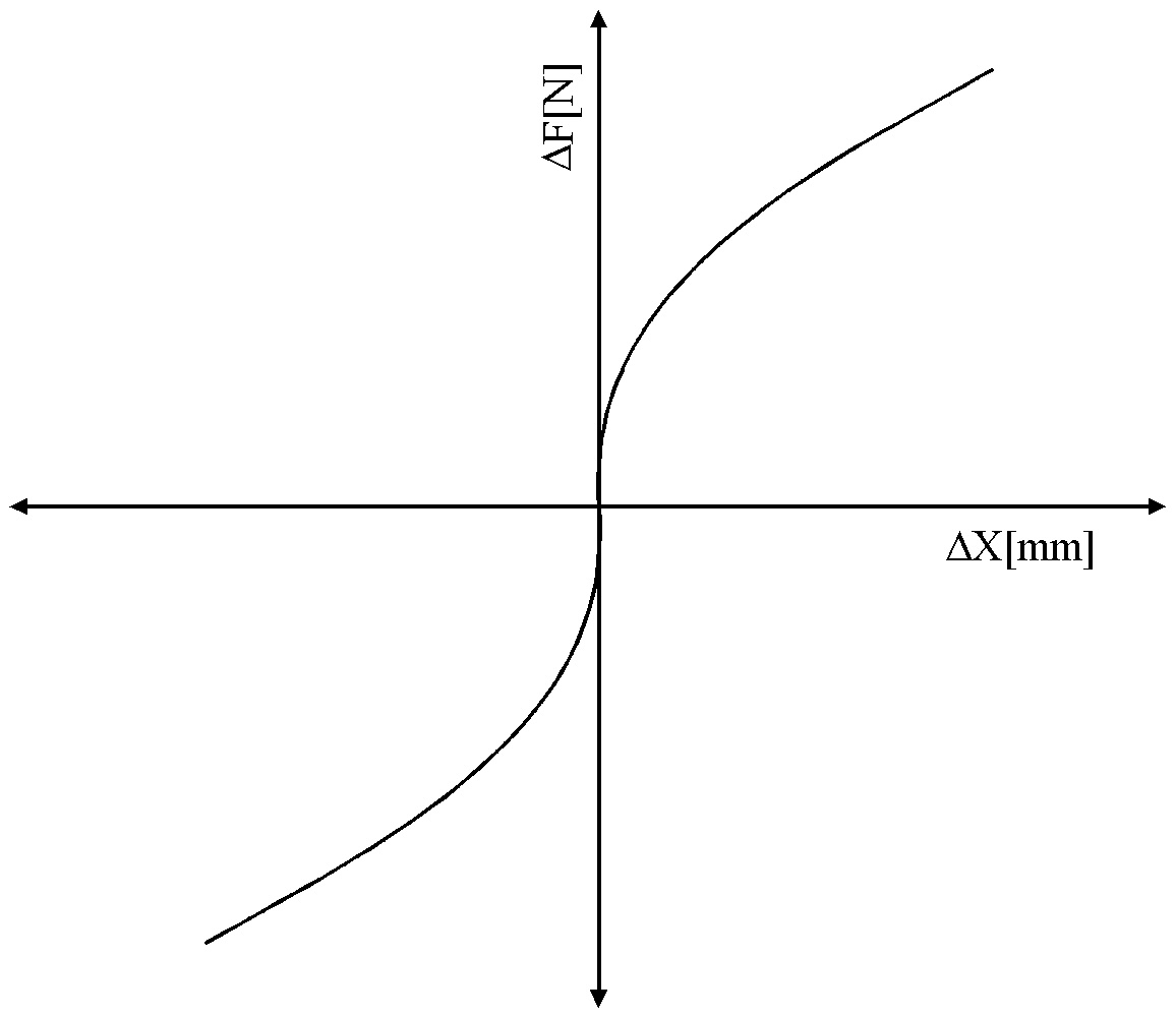
Figure 4. Typical damper spring load/displacement function
B1, B2-Hat
The base stiction force  was estimated to be approximately 2% of the rated force of the linear motor, or 15 [N]. The effects of a change in q on the stiction force was approximated to be 150 [N] with a q of 1 [deg]. The effect of a height differential Dh of 1 [cm] on the stiction force in the tracks was estimated to be 150 [N]. The effect of wave motion on the stiction force was estimated to be was estimated to be approximately 2% of the rated force of the linear motor, or 15 [N]. The effects of a change in q on the stiction force was approximated to be 150 [N] with a q of 1 [deg]. The effect of a height differential Dh of 1 [cm] on the stiction force in the tracks was estimated to be 150 [N]. The effect of wave motion on the stiction force was estimated to be  at the maximum tilt angle. at the maximum tilt angle.
To Summarize:
= 15
Ab= 6000
 = 0.5 = 0.5
Bb= 10000
 = 0.5 = 0.5
O= 10/
 = 0.5 = 0.5
Disturbance Generation Parameters
There are two disturbance signals in the simulation. The first signal models the change in height between the upper and lower tracks, the second signal models the effect of wave motion on the momentum of the handler mass.
For the height disturbance:
- The range of height differential Dh as defined by Orbital Research is given as +/- 1 [cm]. Therefore:
- The frequency of the height disturbance as defined by Orbital Research is given as +/- 2 [Hz]. Therefore:
For the momentum disturbance:
- The max. frequency of the ocean wave motion as defined by Orbital Research is given as +/- 0.1 [Hz]. Therefore:
- The maximum magnitude of the force disturbance is a function of the handler mass, and the maximum angle of tilt in the direction of the carriage motion. The maximum tilt angle of seas with a wave frequency w2 of 0.1 [Hz], a maximum height HW(MAX) = 30 [m], and a wavelength LW equal to 10 times the height (worst case) is given as:
 The momentum force due to this is given as The momentum force due to this is given as  , therefore , therefore 
(split the loading between 2 drives)
SIMULATION STRUCTURE
Overview
The simulation is composed of three main sub-systems: The controller sub-system, the plant sub-system, and the referencing sub-system as shown in Figure 5.
Figure 5. Simulation Main Block Diagram
Reference Generation
The reference generation used in the simulation is based on the generation of an S-curve speed reference. The s-curve speed reference is then integrated to get the position reference. The derivative of the speed reference is multiplied with the load mass to provide the inertia/momentum compensation or force feed-forward signal. Figure 6. illustrates this concept.
Figure 6. Sample reference generation set.
It is intuitively obvious that a set of equations can be derived to describe the above reference profile (i.e. position, speed, and torque which is proportional to acceleration) based on a user specified parameter set. The assumption that there is symmetry in the profile must be made to simplify the generation of the equations. Figure 7. represents a typical speed profile (or pattern) for a run where the percentage of the run where jerk is non-zero is less than 50%.

Figure 7. Constituent Parts of a Position Profile
Assuming there is 1/4 symmetry in the jerk profile in Figure 9. (i.e T1 = T3 = T5 = T7 = Tg and T2 = T6 = Ta ), the following equations can be derived:
 (2.1) (2.1)
 (2.2) (2.2)
 (2.3) (2.3)
 (2.4) (2.4)
combining (1.1) through (1.4) yields the following equation set:
 (2.5a) (2.5a)
 (2.5b) (2.5b)
 (2.5c) (2.5c)
 (2.5d) (2.5d)
 (2.5e) (2.5e)
Given any 4 of the 5 variables, The equations in (2.5) can be used to find the unknown variable.
Plant sub-system
The plant sub-system is a block diagram of Eq’s (1.1) through (1.8) in Chapter 1 and is shown in Figure 8.
Figure 8. Plant Block Diagram
Note that on the acceleration monitoring signals a set of 100 [r/s] lag filters is included to remove high frequency noise. Similarly on the position feedback a set of 200 [r/s] 2nd order Butterworth filters is implemented. This is typical of the type of anti-aliasing filter that is found in most feedback devices. The sub-systems found within the Plant block diagram are described below.
B1_hat Block Diagram
B2_hat (Figure 9.) is identical to B1_hat, with the exception that the signs at the summing junction reflect those shown in Eq. (1.6). Note that, for trouble-shooting purposes, and numerical stability, saturation limits of +10/-10 (+/- 1000% of the fixed static friction offset ) are included on the q and H_hat static friction force computation. This ensures that the simulation remains numerically bounded at all times.
Figure 9. B1_hat Block Diagram
K1,K2 Block Diagrams
(Figure 10.) K2 is identical to K1. Note that saturation limits +0.5/-0.25 (+ 50% to - 25% of the base spring constant K) are also included on the q and H_hat spring constant adjustment calculation to ensure that the simulation remains numerically bounded at all times.
Figure 10. K1 Block Diagram
H_hat Block Diagram
Figure 11., Self-explanatory:
Figure 11. H_hat Block Diagram
Theta Block Diagram
Figure 12. The calculation of q is bounded between +/- 1 [deg] for the same reasons expressed above.
Figure 12. Theta Block Diagram
Controllers Sub-System
Figure 13. Controllers Block Diagram
There are four controllers (Figure 13.) in the system. A set of speed and position controllers for each motor drive. The controllers were implemented in the simulation with discrete s-functions. The s-functions are written with difference equations and internal logic that exactly replicate the behavior of sampled digital control systems, including quantization errors, and are described in Appendix B.
Upper Speed Block Diagram
In Figure 14., normalization constants are used to ensure that the regulator can be tuned in a per-normal manner. The speed reference and feedback are divided by SMAX = 5 [m/s]. The motor specifications state that the motor rated force FMAX = 660 [N] and a max power of 2700 [N]. therefore the LIMIT block limits, LIMUS, are set to  and the normalized force reference is multiplied by FMAX. The Boolean limit plus and limit minus signals are fed out of the speed loop block to be or’ed with the limit plus and limit minus signals in the position regulator (Figure 16.). This ensures that both PI regulator integrators are clamped if the speed loop saturates. and the normalized force reference is multiplied by FMAX. The Boolean limit plus and limit minus signals are fed out of the speed loop block to be or’ed with the limit plus and limit minus signals in the position regulator (Figure 16.). This ensures that both PI regulator integrators are clamped if the speed loop saturates.
Figure 14. Upper Speed Block Diagram
Lower Speed Block Diagram
The lower speed loop block diagram (Figure 15.) is identical to the upper speed loop block diagram, with the addition of some uncertainty in the force reference. The inclusion of this uncertainty enables the simulation to mimic the asynchronous behavior of the two digital control systems. The uncertainty in the reference is bounded between +/- 1 [ms].
Figure 15. Lower Speed Block Diagram
Upper Position Block Diagram
Figure 16. Upper Position Block Diagram
The upper and lower position loop block diagrams are identical. The Lead/Lag in the feedback of the position loops are disabled (RESET = 1). The LIMIT block limits are set to ensure that the position loop does not command more than a 10% vernier to speed loop (i.e. LIMUP =0.1, implies that there will be no more than a 10% of rated speed increase in the speed reference due to control action by the position loop). The Boolean limit signals from the speed regulators (Figure 14,15) are or’ed with the position loop regulator limit signals, to ensure that both the speed and position loop PI integrators are clamped, to prevent wind-up, if the speed loop saturates.
CHAPTER 3
RESULTS
Overview
For each approximate 2 [m] run result, the following plots are included:
- Handler Position error [cm]
- Speeds v0, v1, v2, [m/s]
- K1, K2, Damper Forces [N]
- F1, F2, Motor Forces [N]
The following simulations are investigated:
To demonstrate the effect of damper stiffness (OT, ND – Fig. 17 - 24)
- K = 1000 [N/mm](very stiff dampers)
- K=10 [N/mm] (very sloppy dampers)
To demonstrate the effect of Tuning (ND, K=100 [N/mm] – Fig. 25 - 32)
- w
co(spd) = 50, wco(pos) = 25 (optimal tuning)
- w
co(spd) = 5, wco(pos) = 1 (very poor tuning)
To demonstrate the effect of a height disturbance (OT, K=100 [N/mm] – Fig. 33 - 36)
To demonstrate the effect of wave motion (OT, K=100 [N/mm] – Fig. 37 - 40)
To demonstrate the effect of both wave and height variations (Fig. 40 - 48)
- D
h = +/- 1 [cm], Bv = 400 [N] (otimal tuning, K=100 [N/mm])
- D
h = +/- 1 [cm], Bv = 400 [N] (poor tuning, K = 100 [N/mm])
Finally a set of results (Fig. 49 – 52) were included to show the need for adequate softening in the speed reference. The previous results were conducted with 75% "s" in the speed reference (i.e. only 25% of the speed reference was linear). The set used to demonstrate a low "s" response is the same as the set (K=100 OT, WHD) but with only 5% of "s" in the reference.
Note: The position error is the error between the handler position and the reference, and NOT the error in the position loop itself. Due to the elasticity in the dampers, there will be a steady state error in this value in the presence of a wave induced momentum disturbance force (see Fig. 49 – 52)
Set Up Parameters
The following are the basic plant set-up parameters:
% Masses [kg]
m0= 2;% Top Carriage mass [kg]
m1= 220;% Turret mass [kg]
m2= 2;% Lower Carriage mass [kg]
%Damper damping factor
B1= 1000;% B1 Damping co-eff. [N*s/m]
B2= 1000;% B2 Damping co-eff. [N*s/m]
%H_hat
h = 1.87;% height [m]
A = 0 or 0.01;% max height deviation [m]
w1= 2;% height sinusoidal dist. freq. [Hz]
%K1,K2
K= 10,100 or 1000;% Base K1,K2 Spring Constant [N/mm]
a= 0.5;% K1,K2 Theta_hat exponent []
AK= 10;% K1,K2 Theta_hat exponent gain []
b= 0.5;% K1, K2 H-hat exponent []
BK= 20;% K1,K2 H-hat exponent gain []
%B1_hat,B2_hat
B_hat= 15;% Base B1,B2_hat Force Constant [N]
a_hat= 0.5;% B1,B2_hat Theta_hat exponent []
AB= 6e3;% B1,B2_hat Theta_hat exponent gain []
b_hat= 0.5;% B1,B2_hat H-hat exponent []
BB= 1e4;% B1,B2_hat H-hat exponent gain []
w2= .1;% B1,B2_hat Disturbance Frequency [Hz]
Bv= 0 or 400;% B1,B2_hat Disturbance Frequency force [N]
OB= 10/Bv;% B1,B2_hat Disturbance stiction gain []
th_hat= 0.5;% B1,B2_hat th_hat exponent []
The following nomenclature is used in the Figure descriptions:
OT:Optimal tuning (40 [r/s] speed loop and [25&20 [r/s] pos. loop bandwidths).
PT:Poor tuning (10 [r/s] speed loop and [2.5&3 [r/s] pos. loop bandwidths).
ND:No disturbances.
HD:Height disturbance included.
WD:Wave momentum disturbance included.
HWD:Wave and Height disturbances included.
Damper stiffness (optimal tuning, no disturbances)
Figure 17. Handler Position error [cm] K=1000, OT, ND
Figure 18. Speeds v0, v1, v2, [m/s] K=1000, OT, ND

Figure 19. K1, K2, Damper Forces [N] K=1000, OT, ND
Figure 20. F1, F2, Motor Forces [N] [K=1000, OT, ND
Figure 21. Handler Position error [cm] K=10, OT, ND
Figure 22. Speeds v0, v1, v2, [m/s] K=10, OT, ND
Figure 23. K1, K2, Damper Forces [N] K=10, OT, ND
Figure 24. F1, F2, Motor Forces [N] K=10, OT, ND
Tuning (no disturbances)
Figure 25. Handler Position error [cm] K=100, OT, ND
Figure 26. Speeds v0, v1, v2, [m/s] K=100, OT, ND
Figure 27. K1, K2, Damper Forces [N] K=100, OT, ND
Figure 28. F1, F2, Motor Forces [N] K=100, OT, ND
Figure 29. Handler Position error [cm] K=100, PT, ND
Figure 30. Speeds v0, v1, v2, [m/s] K=100, PT, ND
Figure 31. K1, K2, Damper Forces [N] K=100, PT, ND

Figure 32. F1, F2, Motor Forces [N] K=100, PT, ND
Height disturbance (optimal tuning, K=100 [N/m])
Figure 33. Handler Position error [cm] K=100, OT, HD
Figure 34. Speeds v0, v1, v2, [m/s] K=100, OT, HD
Figure 35. K1, K2, Damper Forces [N] K=100, OT, HD
Figure 36. F1, F2, Motor Forces [N] K=100, OT, HD
Wave motion (optimal tuning, K=100 [N/m])
Figure 37. Handler Position error [cm] K=100, OT, WD
Figure 38. Speeds v0, v1, v2, [m/s] K=100, OT, WD
Figure 39. K1, K2, Damper Forces [N] K=100, OT, WD
Figure 40. F1, F2, Motor Forces [N] K=100, OT, WD
Wave and height variations
Figure 41. Handler Position error [cm] K=100, OT, WHD
Figure 42. Speeds v0, v1, v2, [m/s] K=100, OT, WHD
Figure 43. K1, K2, Damper Forces [N] K=100, OT, WHD
Figure 44. F1, F2, Motor Forces [N] K=100, OT, WHD
Figure 45. Handler Position error [cm] K=100, PT, WHD
Figure 46. Speeds v0, v1, v2, [m/s] K=100, PT, WHD
Figure 47. K1, K2, Damper Forces [N] K=100, PT, WHD
Figure 48. F1, F2, Motor Forces [N] K=100, PT, WHD
The Effect of "s" in the Speed Reference
Figure 49. Handler Position error [cm] K=100, PT, WHD (5% "s’)
Figure 50. Speeds v0, v1, v2, [m/s] K=100, PT, WHD (5% "s’)
Figure 51. K1, K2, Damper Forces [N] K=100, PT, WHD (5% "s’)
Figure 52. F1, F2, Motor Forces [N] K=100, PT, WHD (5% "s’)
OBSERVATIONS AND CONCLUSIONS
OBSERVATIONS
The use of a linear motor, and a drive that is capable of obtaining 40 – 50 [r/s] bandwidth on the speed loop, and 20 – 30 [r/s] bandwidth on the position regulators, along with speed and momentum compensation feed-forward signals, will provide adequate positioning performance in the positioning loops, over the range of modeled disturbances. One distinct advantage to using a linear motor is the removal of backlash from the drive train. Backlash and torsional wind-up are the factors that most typically limit speed loop bandwidths in large (over 50 [kg] reflected mass) systems.
The modeled stiction force disturbances, as a function of a change in rail separation distance, misalignment of upper and lower tracks, and a change in normal loading as a result of ocean wave motion, were probably more severe than can be expected in the physical application. Based on this observation I am fairly confident that the system should perform adequately in terms of positioning the carriages. The positioning of the handler, which is attached to the carriages by the carriage dampers, is a separate issue, and discussed below.
It should be noted that the effects of motion in the other two degrees of freedom (i.e. side-to-side, and torsional loading forces) and their effect on the stiction force in the rails have not been investigated. Overload conditions may occur in the drive under extreme conditions. In the one degree of freedom model, a total of 300 – 400 [N] of losses per motor were possible as a result of stiction forces with a +/- 1 [cm] deviation in height, a +/- 21o angular shift in the translational direction, and a misalignment of 1o between the railings. If these stiction force estimations are correct, and given that the motors to be used are rated at 660 [N], not much headroom is left to accelerate the mass, and compensate for other stiction forces, in a high duty-cycle operational mode. Based on these observations, overloading may prove problematic when the system is implemented on board a ship. Again, this will depend on the amount of stiction in the system under expected ocean-going operating conditions.
The simulations performed to demonstrate the effect of wave motion on the handler momentum showed that the error in the handler position is a function of the ship angle from horizontal. At 20o - 25o (worst-case) the deviation with a 100 [N/mm] spring constant was approximately 4 [mm]. This error is directly proportional to the stiffness of the dampers. If dampers with 1000 [N/mm] spring constants were used, the deviation would only be 0.4 [mm]. Depending on the alignment requirements for both the grabber and the mechanism that loads the projectile into the firing chamber, the stiffness of the damper used may have to be re-evaluated based on the expected worst-case ocean going conditions. At the time of this writing, no information was made available with respect to the physical characteristics of the dampers.
Another consideration that must be made with respect to the dampers, is the ability of the dampers to absorb a load shock from a near hit. They cannot be excessively stiff, as this will negate their load shock absorption capabilities. These two conflicting requirements will involve some trade-offs in the choice of the stiffness of the dampers and the expected alignment error in heavy seas. The alignment requirements for the handler should be the starting point for making the trade-off decisions.
Variation in system natural frequencies due to variation in the damper spring constant should not be problematic. Closed loop stability issues as a result of system natural frequency deviations are usually not problematic in positioning systems where the position feedback is taken from a stiff member of the system (i.e. the rails). This appears to be especially true in this application.
Another observation from the simulation that directly affects the alignment of the handler is the effect of the height differential Dh on the positioning error of the handler. It is clear that the combination of both a variation in stiction forces and damper spring constant due to this phenomena will impact the ability of the handler to remain aligned during ocean going operations. Based on these observations, the need for some latitude on the docking mechanism is evident.
The tuning of the two speed and position regulators should be as symmetric as possible. It was found through simulation that the two drive systems tend to "fight" each other when the tuning is not symmetric. Several simulations that were performed using a slaved force reference resulted in a larger deviation in the upper and lower track alignment than was observed with a two-regulator system, although it was not significantly worse. The application may reveal that unmodeled dynamics and non-linear loading factors in the physical implementation will produce a lower misalignment with the slaved regulator structure than with the parallel regulator structure. This should be investigated more closely during the system start-up.
The scope of this study does not include sequencing issues, however it should be noted that the safety issues discussed at the meeting on March 22nd need to be addressed, before the unit is tested.
CONCLUSIONS/RECCOMENDATIONS
- The set-up of the drives should be configured for both a slaved, and a parallel regulator configuration. Both configurations should be tested during system start-up.
- The speed loops should be step tested with load attached, for a 40 – 50 [r/s] bandwidth (time to peak of approx. 60 [msec]). Care should be taken to ensure that no saturation occurs in the loops when the step test is performed.
- The position loops should be step tested for a response of 20 – 30 [r/s] bandwidth (time to peak of approx. 120 [msec]). Care should be taken to ensure that no saturation occurs in the loops when the step test is performed.
- The feed-forward speed, and momentum compensation signals should be verified to be scaled correctly by running the system open speed, and position loop, and checking the response with only the feed-forward signals active (It may be that the drive configuration does not permit this)
- Adequate softening of the references (at least 50% "s") should be used to ensure that stiff torque steps do not excite natural frequencies in the structure.
- The sizing of the dampers w.r.t. their force/deflection characteristics should be carefully investigated. The handler alignment errors that result from working the system while experiencing worst case operating conditions should not affect its ability to perform projectile loading and unloading tasks.
- The docking mechanism should be assessed to verify that it satisfies the need for latitude during operation in an environment that includes the disturbances modeled in this study.
| 